MACS Matchmaker

Experiment Design

Plan a MACS Matchmaker measurement: choose what to immobilize, set up assay phases, build injections in the Advanced Planner, and configure flow and buffer conditions, including the R_max and ligand density the assay is planned around. Pickup volume is in the expandable section at the bottom. Regeneration conditions have their own page.

The guided experiment wizard

The wizard writes a complete injection plan from a handful of answers, and everything it produces stays editable afterwards in the Advanced Planner. Use the phase templates below to build other designs in the Advanced Planner.

1 · Goal

Name the experiment, optionally tag and describe it, and pick what it is for. Four goals are offered:

Binding Kinetics & Affinity — then SCK or MCK. See Assay Types for which one fits.
LOD — a serial dilution series with leading blanks.
Scouting — a short run that tests ligand immobilization, optionally with backfilling and a binding injection. Use it before committing a full kinetic design to an unproven surface.
Concentration Determination measures a calibration series for each standard and a dilution series for each unknown.

2 · Instrument

Defaults arrive from the goal, so this step is usually a confirmation. It covers chip format and multiplexing, the flow chamber configuration, the sensor architecture, and the well plates on each side of the autosampler. Export and image settings sit here too, including the export frequency and whether fluorescence images are written.

3 · Samples

Ligands, analytes and regeneration solutions, each with a name and a free note for concentration. Autoplace Ligands distributes them across the chip by multiplexing group; Inject as Pool injects a group together, and backfilling ligands are never pooled.

What the analyte is for follows the goal: titrated over the ligands for kinetics, titrated to characterise the detection limit for LOD, optional for scouting, and for Concentration Determination either a calibration standard or an unknown sample, chosen per row in the Calibration and Unknown columns. Skip immobilization is unavailable for that goal.

4 · Method

The parameters specific to the goal, above all the concentration series. Enter it either as an explicit range or as an expected $K_D$ that the wizard expands into a sweep around it — the same choice the Single Cycle Kinetics dialog offers. A timeline previews the run as configured.

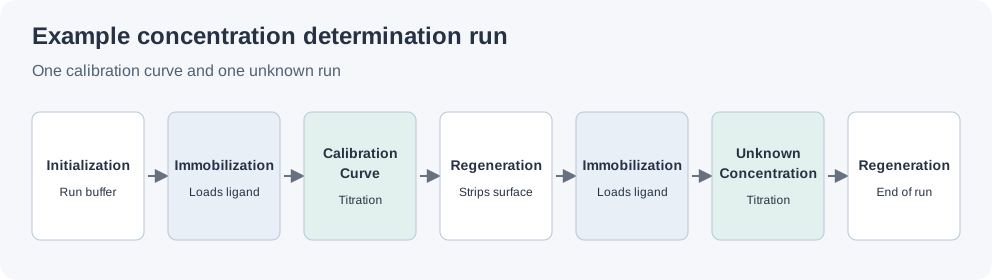
Concentration Determination generates one Calibration Curve titration per calibration analyte and one Unknown Concentration titration per unknown, up to 20 of each; both cards list their analyte names. Without unknowns, only calibration curves are measured. Without calibration analytes, no curve is measured and the unknowns are later evaluated against an existing calibration curve from another measurement. Dilution settings apply to each unknown's own series, from a blank up to the undiluted sample.

Initialization starts the run with 3 min of running buffer at 300 µL/min. Each Calibration Curve and Unknown Concentration phase contains Titration groups and follows its own Immobilization phase, with a Regeneration between titrations. Tick Covalently immobilized ligand to regenerate after each Immobilization too; a DDI ligand, which that regeneration would strip, leaves it clear. The final regeneration includes optional trypsin cleanup once, after all titrations.

Example run: Initialization, then Immobilization and Calibration Curve, then Regeneration, Immobilization and Unknown Concentration, closing with a final Regeneration. The calibration and unknown phases contain Titration groups.

5 · Review

Final adjustments to the well plate, then either Save or Save & Prepare Measurement to go straight to the instrument. The saved plan behaves like any hand-built experiment from this point on.

Choosing Ligand and Analyte

The decision of which molecule to immobilize on the mologram (ligand) and which to flow in solution (analyte) affects data quality and interpretation. Consider the following guidelines:

Immobilize the smaller, more stable molecule. A smaller ligand leaves more room for the larger analyte to bind without steric interference. Additionally, larger analytes produce a stronger signal per binding event (more pg/mm² per molecule), improving the signal-to-noise ratio.
Flow bivalent molecules as analyte with caution. A bivalent analyte such as a full IgG can bind two ligands at once, so consider a monovalent fragment (Fab) or a lower ligand density where a clean 1:1 fit matters. The avidity mechanism and its effect on the fit are covered under Bivalent analyte and avidity.
Preserve ligand activity. The immobilized molecule must remain functional after coupling. For click chemistry chips, covalent attachment via TCO–Tz/Me-Tz may affect protein folding if the label is placed near the binding site. For DDI chips, the DNA conjugation strategy is generally milder and more predictable.
Practical constraints. Immobilize the molecule that is available in smaller quantity (less material is needed for surface immobilization than for flowing multiple concentrations). Flow the molecule that is easy to prepare in a dilution series.

Assay Phases

Each assay type starts from a phase template. For the full list of templates and what each one contributes, see The phases a plan is built from on Assay Types; the guidance below is for the phase-specific design choices. For all flow rates and injection volumes, see Recommended Flow Parameters.

Baseline

Allows the system to stabilize before the first relevant injection. Run the running buffer until the baseline is flat.

Association & Immobilization

Frontfilling and backfilling can be configured with the Immobilization template when appropriate (see Immobilizations).
In the guided experiment wizard, choosing the [Oligo|Oligo] sensor architecture adds an empty ligand row to the Samples step with its placement set to Backfilling.
For titration experiments (LOD, SCK, MCK, …) the sample/target must be defined as the Analyte.
To tune ligand surface density on DDI chips, see Ligand Density vs. Mass Transport Trade-Off.

Kinetics Injections

Use a kinetics phase template when it matches your experiment.
Typical durations: 2 min association, 2 min dissociation.

Scouting

Scouting confirms that an assay works — the ligands immobilize, backfilling behaves as expected, and the analyte binds — before a full experiment is committed to the instrument. Its cycle structure, pooling and options are covered under Scouting on Assay Types.

Limit of Detection (LOD)

Experimental setup for LOD measurements. For analysis parameters and the LOD calculation method, see LOD Evaluation.

Add a Limit of Detection phase.
Blanks: the phase requires at least three, and more than five is the usual choice — they set the noise the detection limit is measured against.
Typical durations: 2 min baseline, 5 min association.
Flush sample after association: 200 µL flush at 200 µL/min.
Use the same flow rate for association and dissociation to minimize noise impact.

Concentration Determination

Choose Concentration Determination in the guided wizard, or add Calibration Curve and Unknown Concentration phases in the Advanced Planner, where each dialog writes the Immobilization phase in front of the titration it creates. See Concentration determination on Assay Types for how to plan and run it.

Controls and replication

What runs alongside the sample decides what its result can be compared against. Each control below answers a different question; which of them a given assay needs follows from what could plausibly go wrong with it, not from a fixed list.

Controls

Blank injection. Run buffer through the same injection path, so that injection artifacts and buffer mismatch appear on their own rather than inside a binding response.
Matrix blank. For serum, plasma, lysate or conditioned media, inject the matched matrix without analyte. This is what tells you the backfilling is actually suppressing the coherent background, rather than that you assumed it.
Non-binding mologram. A chemically comparable ligand or bare adapter, to separate what the analyte does to your ligand from what it does to the surface chemistry carrying it.
Positive control. A ligand–analyte pair of known activity, which distinguishes a failed assay from a genuine non-binder. Most valuable when transferring an assay or working up a new surface.
Reference sample. One stable sample repeated across runs, so drift in the surface or the instrument is visible as something other than a surprising result.

Replication

Molograms assigned to the same condition on one chip are technical replicates of the combined surface, fluidic and readout process: their spread covers spot-to-spot surface preparation, local chip variation, fluidic variation and optical readout, which is more than readout precision alone. What it does not cover is everything upstream of the chip, so averaging more of them narrows an interval around whatever that one preparation happened to give.

An independent preparation replicate repeats the surface and sample preparation — a fresh chip, freshly prepared reagents — and is what a claim about the assay rests on. A biological replicate repeats the biological source: a different donor, culture or animal, and is what a claim about a population rests on. The three answer different questions and are not interchangeable; report which one a stated spread came from.

How many to allocate per condition is an assay-development answer, traded off against the multiplexing the chip has to spend elsewhere. Distribute replicates and controls across the layout rather than clustering them, so that a local surface or fluidic effect shows up as disagreement between positions instead of hiding inside one block.

Exclusions

Decide what disqualifies a mologram before you fit — a failed immobilization, a visible artifact over the fitted interval, a fit that does not converge. Applying a criterion chosen after seeing the result is how a data set becomes unfalsifiable, and an inconvenient value is not by itself a reason to drop one. Record which were excluded and why; the evaluation keeps the rejected fits and their reasons for exactly this.

Building Phases in the Advanced Planner

Charts below the injections preview the plan over time: the flow rate with the sample on the sensor, and — for plans with immobilization — the ligand immobilizations the run passes through. Their time axis ends at the estimated runtime of the plan, the same estimate the measurement queue reports, so a command covers its contact time together with the preparation, delivery and flushing that separate it from the next one.

Titration Series

When planning an experiment, injections are organized into phases. One such phase type is the 'Titration Series'. To use the Titration Series, follow the steps outlined below:

Create a new sample: This sample will serve as the base for all diluted samples, which are auto-generated by the Titration Series dialog. The color of the base sample will be used to distinguish the diluted samples.
Open the Titration Series dialog: In the 'Injections' section, click on the round plus button to add a new phase and select 'Titration Series'.
Fill in the dialog: Specify the highest concentration, the dilution factor, the number of dilution steps, and the placement of blanks. It is possible to repeat the titration series multiple times by setting the repetitions field. A preview of the injection groups with their respective concentrations will appear in the 'Titration Step' section.
Create the step template: Add commands to the step template. These commands will be replicated in each step with the adjusted concentrations. You can choose from command types 'Run Buffer', 'Inject Titration Sample', and 'Inject Sample'. Use 'Inject Titration Sample' for injecting diluted samples, and 'Inject Sample' for regeneration steps where the same solution is injected at each step.
Press 'Create New Phase': This action creates the new diluted samples and one injection group for each dilution step. Manual adjustments to the injection groups, such as adding more blanks or changing the order of injections, are possible.
Press 'Auto Place Vials': After making adjustments, press the 'Auto Place Vials' button in the 'Well Plates' section to place the vials on the Well Plate. Use drag and drop to move the vials to the desired positions.

For guidance on choosing the highest concentration, dilution factor, and number of steps — particularly when $K_D$ is unknown — see Choosing Concentrations.

Single Cycle Kinetics

For when to use SCK, see Assay Types. To configure it:

Create the analyte sample, then add a Single Cycle Kineticsphase.
Enter an expected $K_D$ to generate the concentration range, or set the start, end, and dilution factor manually. Review the association time and final dissociation time.
Create the phase, inspect the generated injections, and auto-place the vials.

Choosing Concentrations

If the $K_D$ is known, enter it in the dialog and the software will suggest an appropriate concentration range. If the $K_D$ is unknown, use the following guidelines:

Start with a wide range, e.g., 0.1 nM to 1 µM, using a roughly 5-fold dilution series (6–7 concentrations).
Use literature values or prior experiments to estimate the range.
Aim to include concentrations both well below and well above the expected $K_D$ to capture the full binding curve from near-zero to near-saturation.
After a first scouting experiment, narrow the range around the observed $K_D$ for more precise fitting.

Why Concentrations Must Span K_D

A broad 0.1× to 10× $K_D$ series brackets the transition from about 9% to 91% occupancy. The 20–80% window, where the isotherm is most sensitive to $K_D$ , lies around 0.25× to 4× $K_D$ . If all concentrations are too high (well above $K_D$ ), the sensor reaches saturation at every step and the curves become indistinguishable — the fit cannot resolve $K_D$ or $k_{on}$ accurately. If all concentrations are too low (well below $K_D$ ), the responses are small and dominated by noise, making the fit unreliable. A well-designed concentration series includes points that produce clearly sub-saturating responses, near- $K_D$ responses, and near-saturating responses.

Multi Cycle Kinetics

For when to use MCK, see Assay Types. To configure it:

Create the analyte sample, then add a Multi Cycle Kineticsphase.
Configure the concentration sweep and repetitions, then review the baseline, association, dissociation and regeneration commands for each cycle, plus the per-cycle immobilization if the ligand is reloaded after each regeneration.
Create the phase, verify the injection groups, and auto-place the vials.

The same concentration-range logic applies to MCK: span $K_D$ with sub-saturating, near- $K_D$ , and near-saturating points (see Choosing Concentrations).

Injection Commands

Inject and Incubate

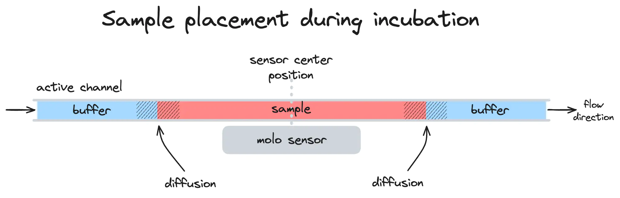
When selecting the pickup volume for the inject and incubate command, consider the effects of diffusion from the autosampler loop. As illustrated in the figure below, a larger volume reduces the impact of diffusion. Both the incubation duration and fluid viscosity influence this process. Given a sensor volume of 3 µL in the single flow chamber, a default value of 30 µL is recommended.

Inject with Alternate Flow

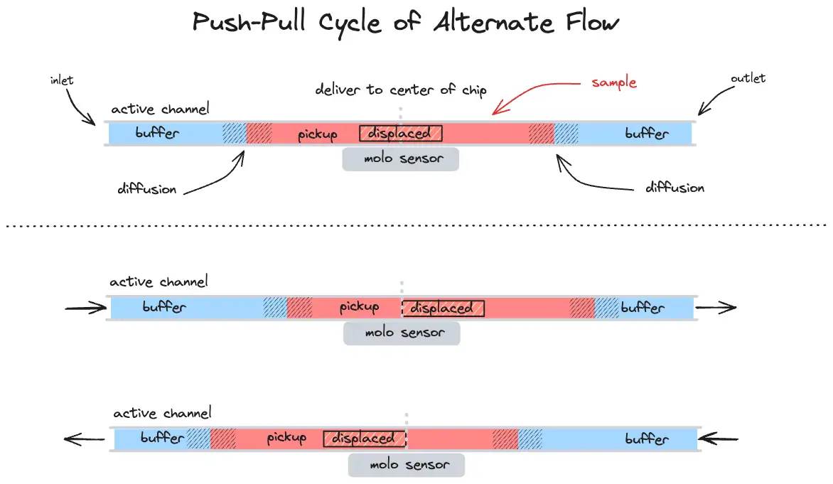
If the sample volume is limited and/or a high flow rate is required, the Alternate Flow incubation mode of Inject and Incubate can be used. This pushes and pulls the sample over the sensor for a specified time. The pickup volume is the amount of sample that is delivered to the sensor. The displacement volume defines how much the sample is pushed forth and back. Both parameters can be set in the command dialog.

Other Commands

Inject Sample: injects a sample. A vial is automatically placed at the next free location and the required volume is calculated when Auto Place Vials is pressed. The required volume equals the injection's pickup volume, which includes the configured additional pickup volume and, for partial-loop pickup volumes from 227 to 250 µL, a non-editable 30 µL loop flush the autosampler needs in partial loop mode. Vial dead volume is not accounted for.
Run Buffer: runs the running buffer for the specified time and flow rate.
Inject from Vial: injects a user-specified volume from a user-specified vial. The vial must be filled with sample before the injection — no auto-placement is performed.
Switch Buffer: changes the running buffer feeding the flow chamber, for a run that uses more than one.

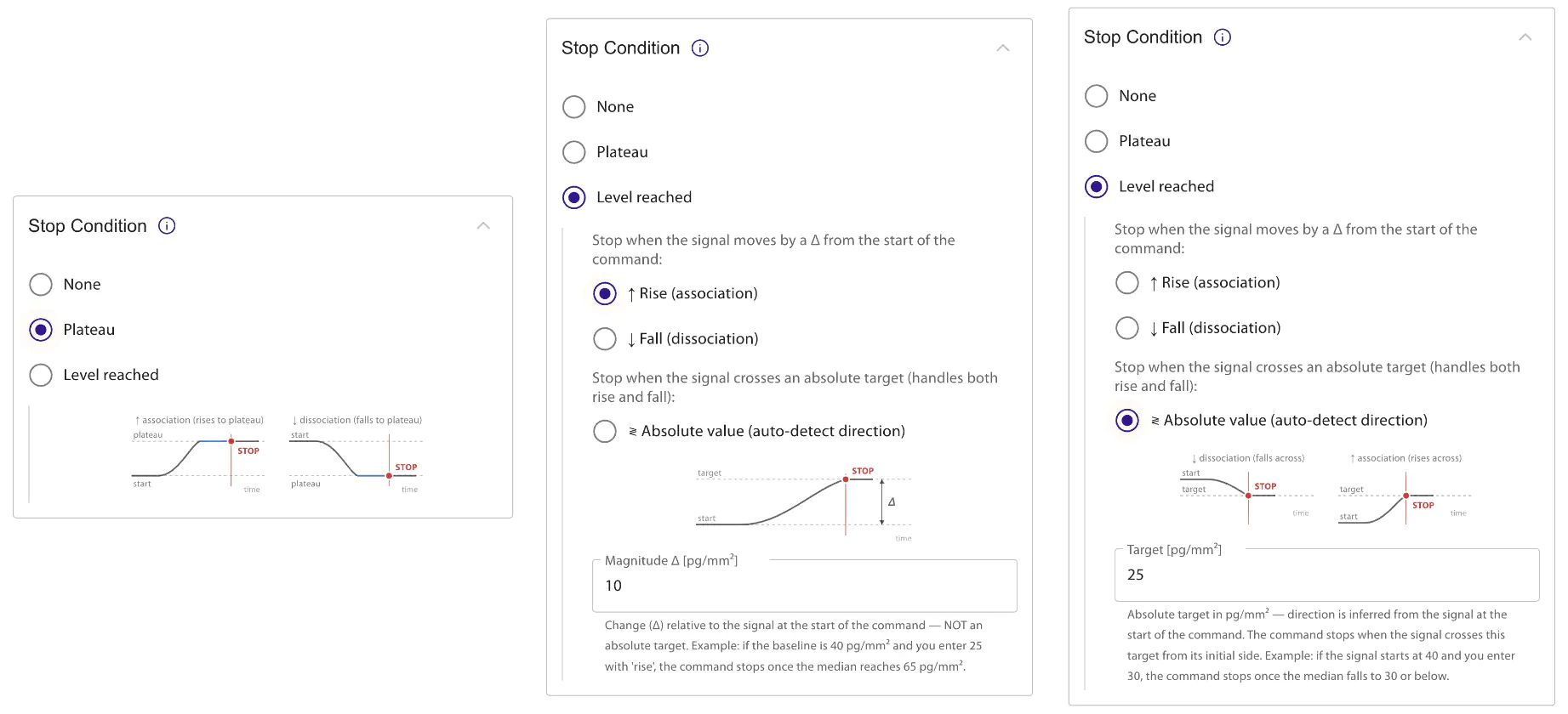
Stop Condition

Each command includes an optional Stop Condition that automatically terminates the command based on specific criteria. There are three selectable stop conditions:

None: Default setting. The command runs until completion unless manually edited or fast-forwarded.
Plateau: Monitors the median coherent mass density of active signal molograms. The system records 10 initial data points, then evaluates whether each of the last 4 points sits within 1% of their median, or within 0.1 pg/mm² of it where the signal is near zero. When this criterion is met, the command fast-forwards.
Level reached: Terminates when the median coherent mass density reaches a configured target. Three sub-options select how the target is interpreted:
- ↑ Rise (association): the value entered is a delta (Δ); the target is starting signal + Δ. The command stops when the most recent points — two at the first check, up to four thereafter — are all at or above the target (in pg/mm²).
- ↓ Fall (dissociation): the value entered is a delta (Δ); the target is starting signal − Δ. The command stops when the most recent points — two at the first check, up to four thereafter — are all at or below the target.
- ≷ Absolute value (auto-detect direction): the value entered is treated as an absolute target in pg/mm² rather than a delta. The direction is inferred from the signal at the start of the command: if the initial 4-sample window sits below the target the command stops on an upcross; if it sits above, the command stops on a downcross.
Examples (Δ-based): if the baseline is 40 pg/mm² and you enter a magnitude of 25 with 'Rise', the command stops once the median reaches 65 pg/mm². With 'Fall' it would stop at 15 pg/mm².
Example (absolute): with an 'Absolute value' target of 5 pg/mm² and an initial signal of ~40 pg/mm² (higher than the target), the command stops when the signal falls to 5 pg/mm² — useful as a safety floor that prevents, e.g., zero-crossing.

Autosampler Injection Modes

The MACS Sampler supports three injection modes. The software automatically selects the best mode based on the programmed injection volume:

Mode	Volume range	Reproducibility	Sample loss
µL Pickup	Up to 227 µL	< 1% RSD	None
Partial loop	227–250 µL	< 0.5% RSD	30 µL (flush volume)
Full loop	500 µL (loop volume)	< 0.3% RSD	530 µL

RSD = Relative Standard Deviation, a measure of injection reproducibility (lower is better).

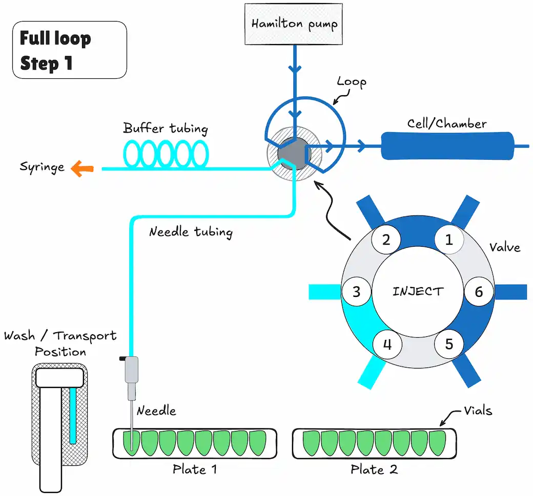
Full Loop Injections

The sample loop is completely filled (quantitatively) with sample. This type of injection results in extremely good reproducibility.

Step 1: At the beginning, the injection valve is in INJECT position. The sample needle with air needle has entered the well or vial. Headspace pressure, applied through the air needle, ensures that no air or vapor bubbles are formed during sample aspiration.
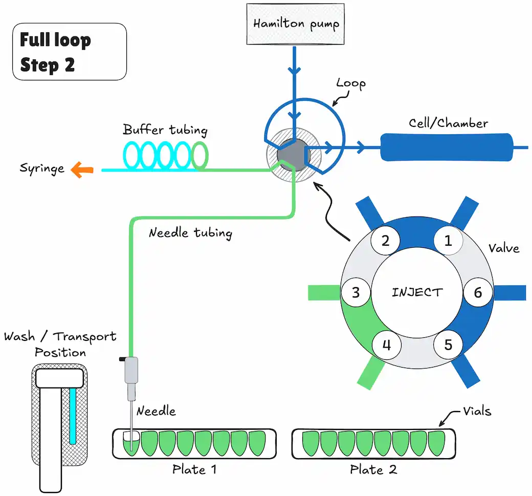
Step 2: The syringe dispenser aspirates the flush volume from the sample well/vial to fill the sample line with sample and remove wash solvent.
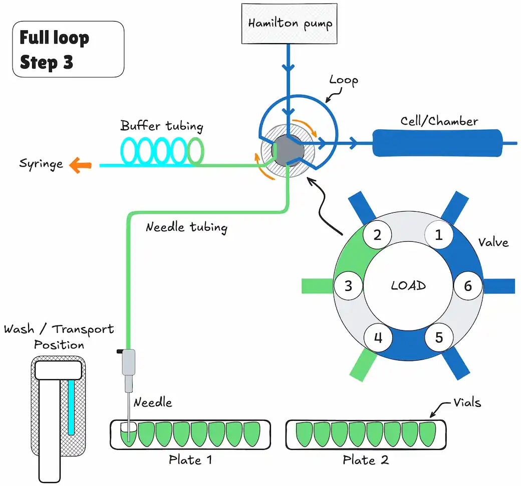
Step 3: The injection valve is switched to the LOAD position, placing a distinct sample plug at the inlet of the sample loop.
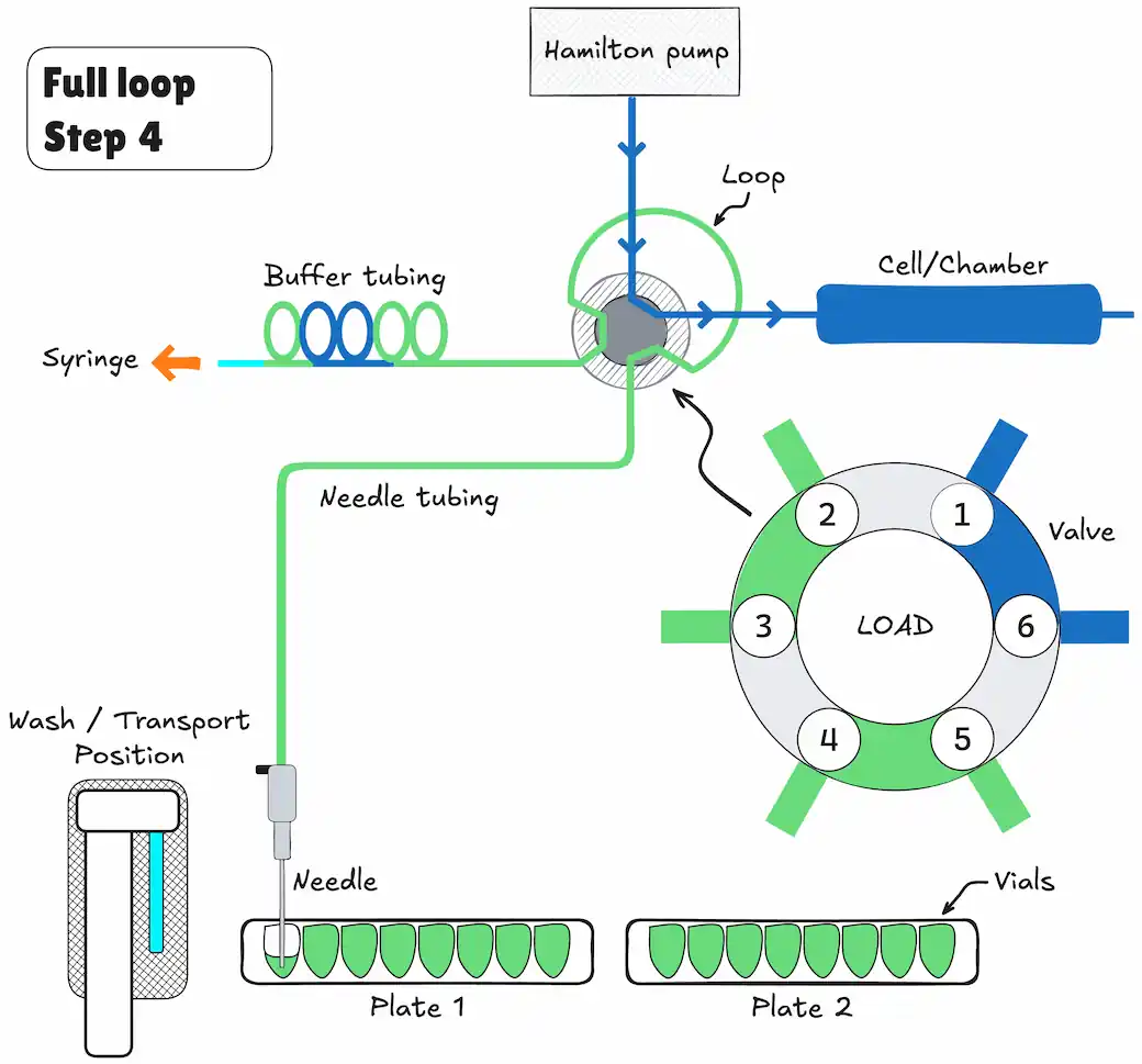
Step 4: The sample loop is quantitatively filled by transporting a number of times the loop volume through the loop, depending on the volume of the loop:
- 3 x loop volume for loops ≤ 100 µL
- 2 x loop volume for loops between 100 µL and 500 µL
- 1.5 x loop volume for loops > 500 µL
Step 5: The injection valve switches to the INJECT position. The sample loop is not part of the HPLC mobile phase flow path: sample is transported to the column. The analysis starts.

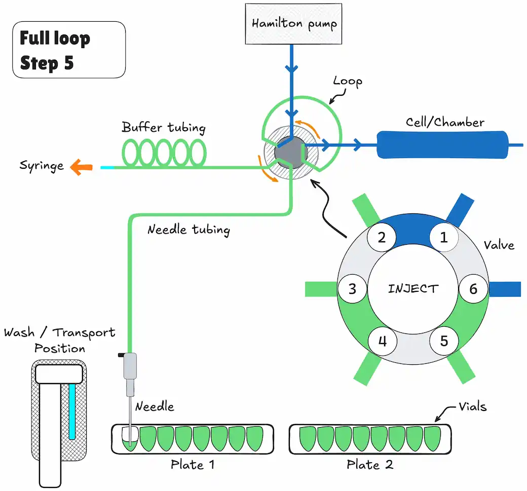
A wash routine is performed after each injection.

Partial Loop Fill Injections

The switching sequence for a partial loop fill injection is:

Step 1: At the beginning, the injection valve is in the INJECT position. The sample needle with air needle has entered the vial/well. Headspace pressure (optional), applied through the outer air needle, ensures that no air or vapor bubbles are formed during sample aspiration.
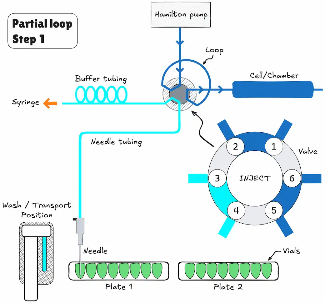
Step 2: The syringe dispenser aspirates the flush volume from the sample vial to fill the sample line with sample and remove wash solvent.
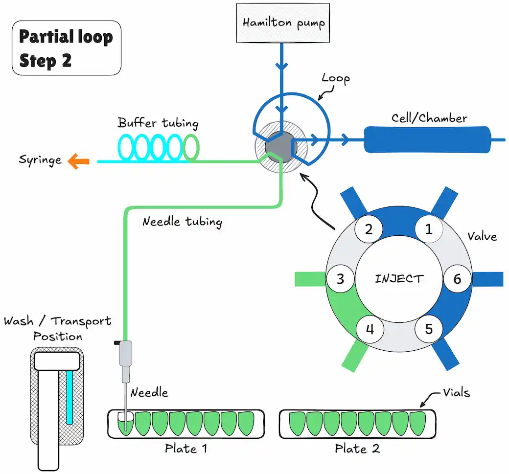
Step 3: The injection valve switches to LOAD, ensuring a distinct sample plug at the beginning of the sample loop.
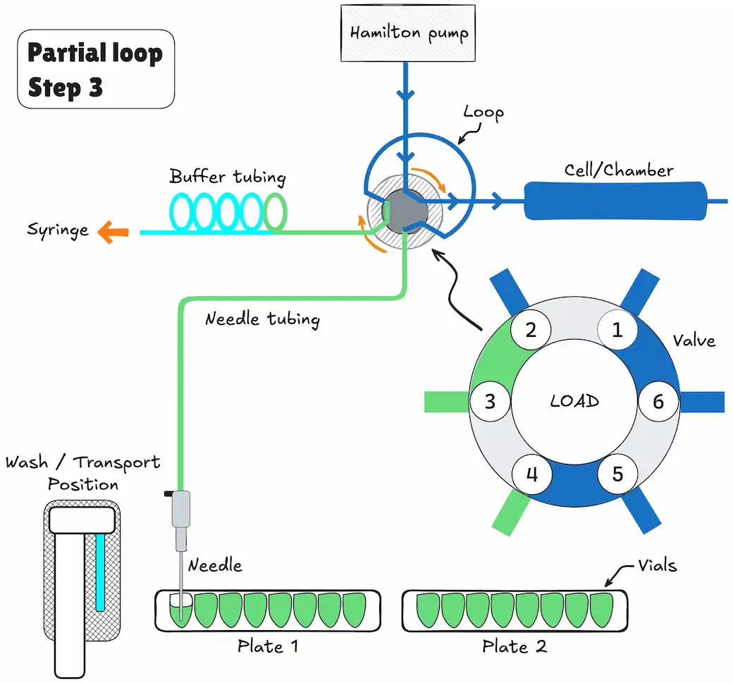
Step 4: The programmed injection volume is now aspirated into the sample loop.
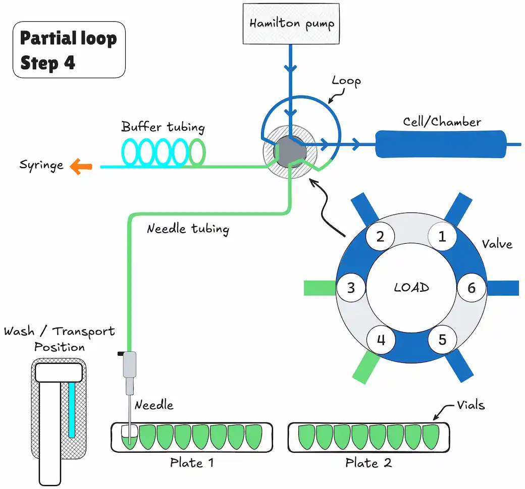
Step 5: The injection valve switches to INJECT. The sample loop is now part of the (U)HPLC mobile phase flow path: sample is transported to the column. The analysis starts.

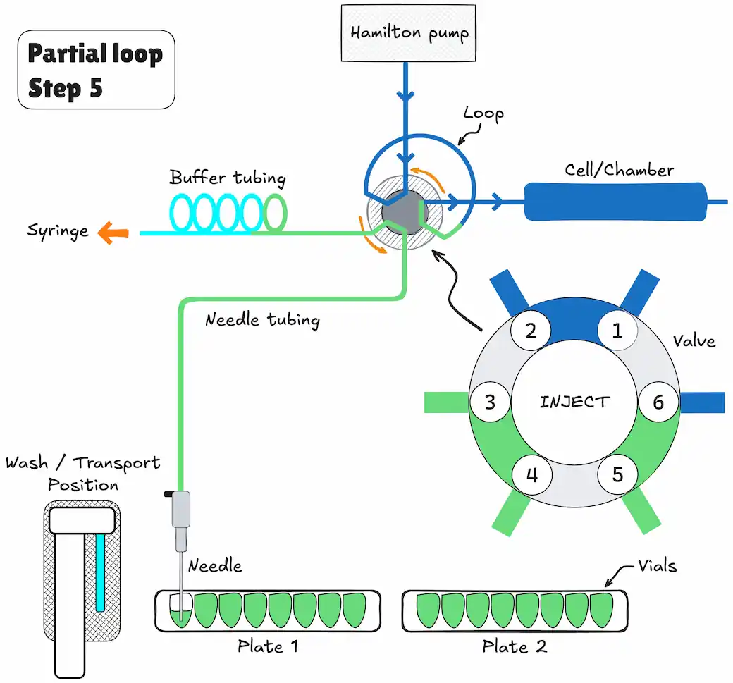
If an injection from the same vial and no wash routine is programmed, the next injection sequence will start with a flush of 50% of the programmed flush volume. Otherwise, it will start with a flush of the programmed flush volume. If the withdrawal of sample for the next injection exceeds the total volume of the sample buffer tubing, the buffer tubing is rinsed before the next injection. The next injection will start with the programmed flush.

µL Pickup Injections

The switching sequence for µL pickup injections is:

Step 1: At the beginning, the injection valve is in INJECT position. The sample needle has entered the transport position.
Step 2: The transport reservoir is filled with wash solvent the programmed amount of times the syringe volume (after a wash or after emptying of buffer tubing). The injector valve remains in INJECT position during fill transport. Please note that the transport solvent needs to be compatible with eluent.
Step 3: For the first injection, the syringe dispenser aspirates a transport plug from the transport position to fill the sample line with transport liquid and remove wash solvents.

Step 4: The needle moves from the transport position to the sample vial. The injection valve switches to LOAD position.
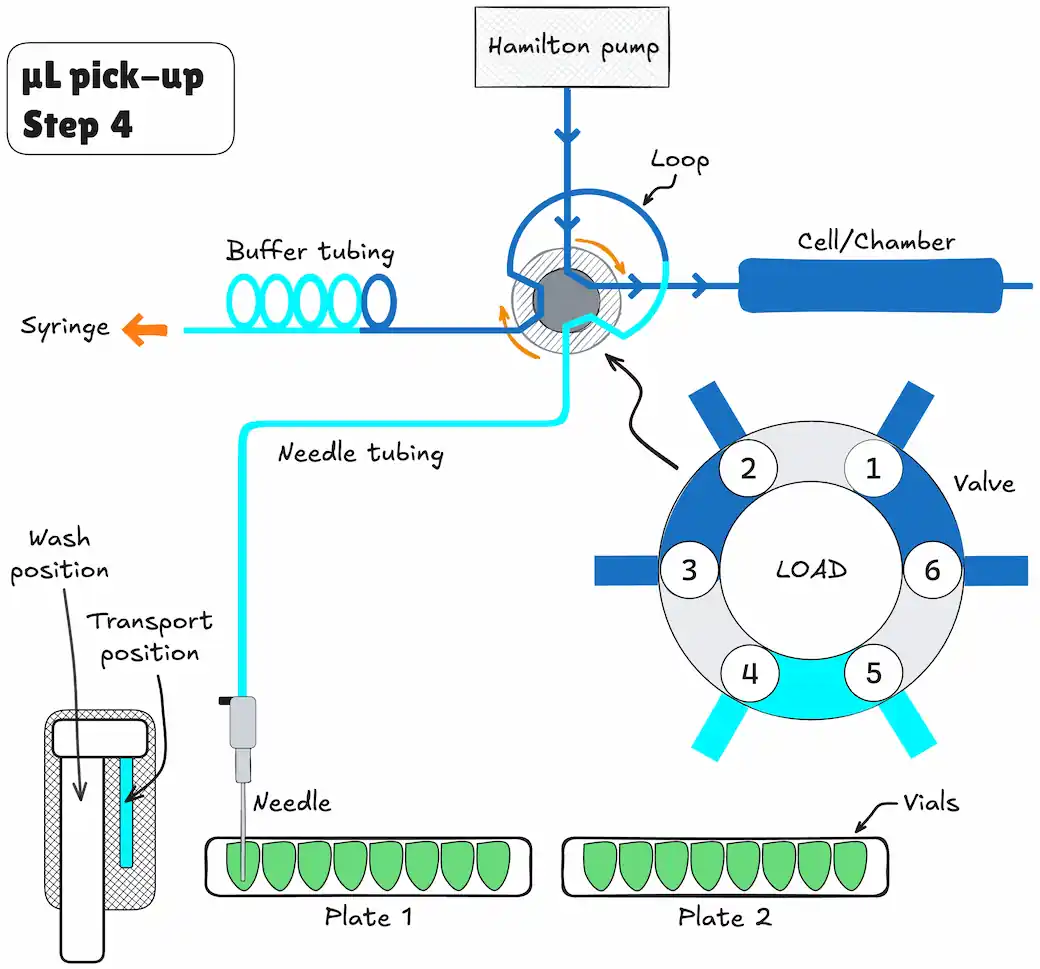
Step 5: The programmed injection volume is aspirated from the sample vial.
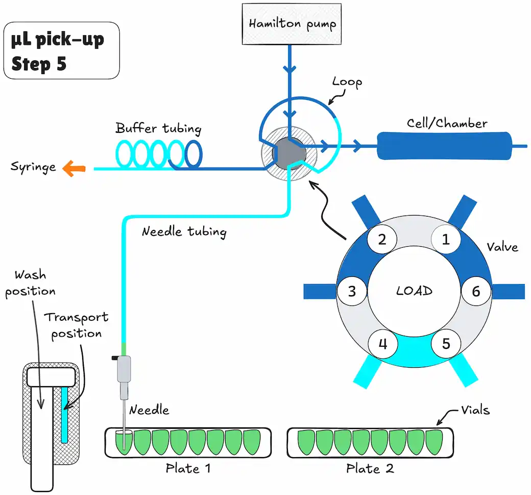
Step 6: The sample needle moves back to the transport position. A second transport plug is aspirated. The sample is quantitatively transported into the loop.
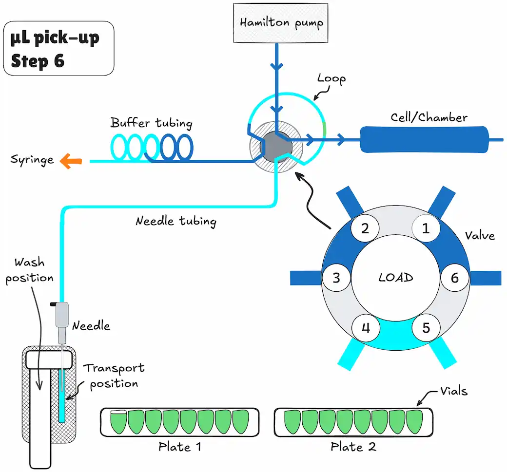
Step 7: The injection valve switches to INJECT. The sample loop is now part of the HPLC mobile phase flow path: sample is transported to the column. The analysis timer starts.

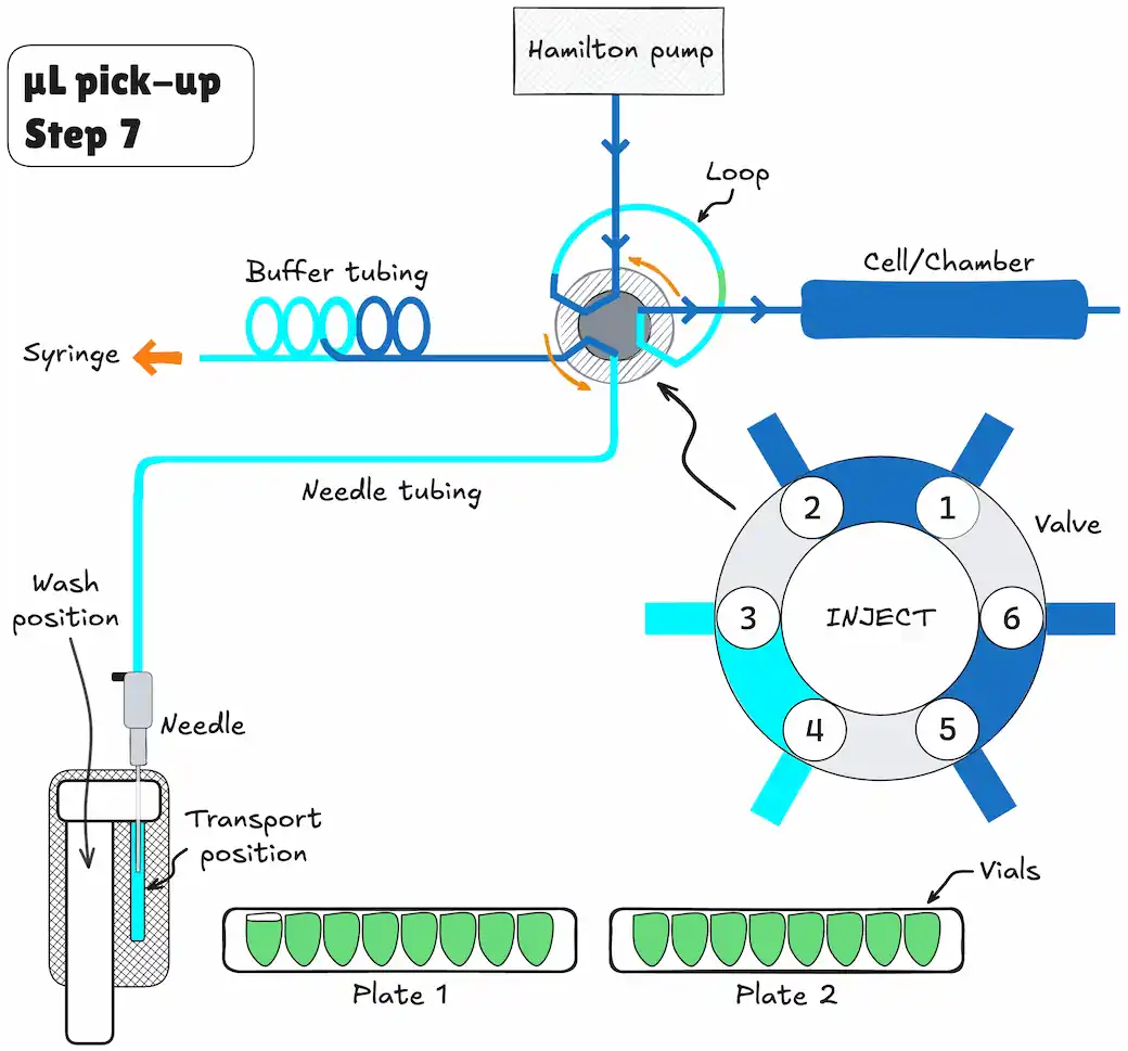
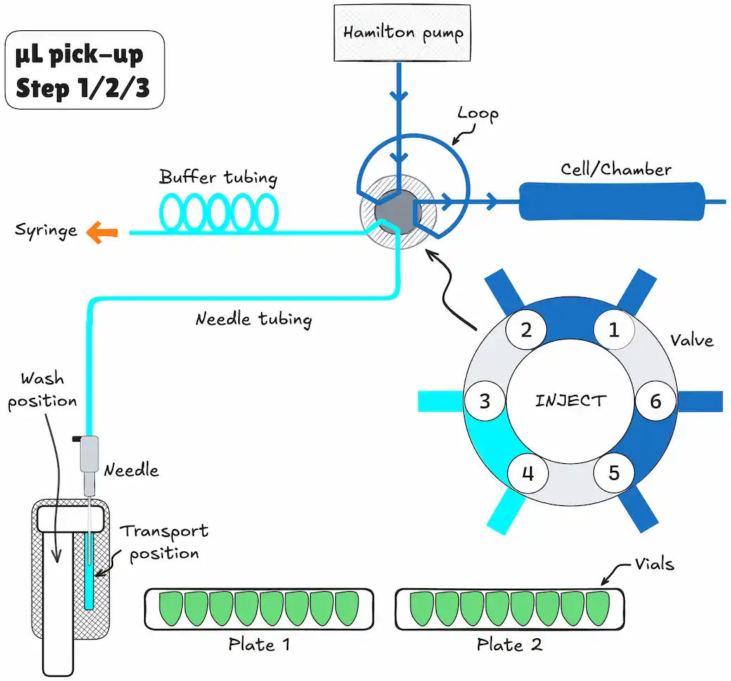
The sequence is repeated for each injection.

Samples and Buffer Recommendations

Focal molography is more tolerant of sample-to-running-buffer mismatch than SPR, so exact matching is not always required.
For quantitative kinetics and whenever bulk effects are visible, still minimize mismatch between running buffer and sample buffer.
Suitable buffers: PBS, HEPES, or Tris-based systems. All buffers should be supplemented with surfactant molecules, such as Tween 20, at a recommended concentration of 0.05% v/v.
Buffers and samples can also contain pre-blocking molecules, such as BSA, casein, or MoloBlock.
For complex media samples, we recommend centrifuging samples and using only supernatant to prevent clogging of the tubing with aggregated sample.
Avoid particulate matter in samples to prevent clogging of the fluidic system.

Recommended Flow Parameters

The MACS Matchmaker is compatible with aqueous solutions from pH 1–13. For flow chamber layouts and mologram counts, see Chip Assembly.

Default values: use the preferred-flow column as the starting point for new experiments, then adjust if sample volume, kinetics, mass transport, or regeneration strength require it.

Phase	Minimum flow	Preferred flow	Notes
Baseline	200 µL/min	300 µL/min	3–5 min to stabilize before the first injection.
Immobilization (DDI)	20 µL/min	20 µL/min	10 min at 100–200 nM ligand concentration.
Immobilization (TCO–Me-Tz / TCO–Tz)	6 µL/min	6 µL/min	~15 min, or until plateau is reached.
Association (kinetics)	30 µL/min	50 µL/min or higher	Use higher flow to reduce mass transport limitations.
Dissociation (kinetics)	100 µL/min	200 µL/min	Higher flow when stronger washout is needed.
LOD association	20 µL/min	Match association & dissociation	Keep association and dissociation flows equal to minimize noise impact.
Regeneration	400 µL/min	400 µL/min	Typically 30 s, followed by 3 min running buffer at 300 µL/min.

Injection volume: use > 90 µL (avoid < 50 µL) to prevent sample dilution from tail diffusion.

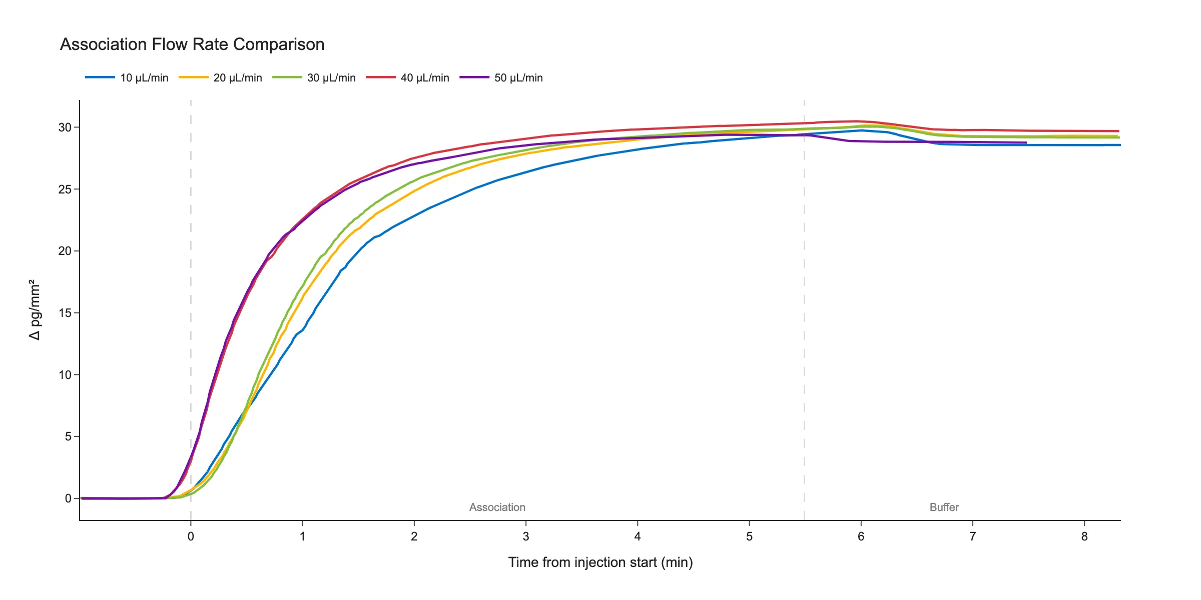
Effect of Flow Rate on Association Kinetics

The overlay below shows the same association phase at different flow rates. If the sensorgram shape changes when you increase the flow rate, mass transport is likely limiting your measurement — continue increasing until the curves overlay.

Association phase overlay at different flow rates

R_max Estimation & Ligand Density Optimization

Predicting the expected maximum response helps assess whether an experiment is performing as intended and guides ligand density choices.

Expected R_max Calculation

The theoretical maximum response for a 1:1 interaction can be estimated from:

R_max,expected = (MW_analyte / MW_ligand) × immobilization level × stoichiometry

where the immobilization level is the capture level observed during ligand immobilization (in pg/mm²), MW values are molecular weights, and the stoichiometry is the number of analyte molecules each ligand can bind (1 for a monovalent ligand). A bivalent analyte such as a full IgG that bridges two ligands lowers it below 1 rather than raising it.

For example, if 20 pg/mm² of a 50 kDa ligand is immobilized and the analyte is a 150 kDa monovalent molecule, the expected R_maxwould be approximately (150/50) × 20 = 60 pg/mm².

Active Fraction Assessment

If the observed R_max from fitting is significantly lower than the calculated R_max,expected, it suggests that not all immobilized ligand is active. Common causes include:

Ligand denaturation during immobilization (especially relevant for click chemistry chips where covalent coupling conditions may affect protein folding).
Unfavorable orientation — binding sites may be blocked or sterically hindered on the surface.
Steric crowding at high ligand densities, where neighboring ligand molecules physically prevent analyte access.

An active fraction of 50–80% is typical for well-optimized assays. Values below 30% warrant optimization of immobilization conditions.

Ligand Density vs. Mass Transport Trade-Off

Higher ligand density produces a stronger signal but increases the risk of mass-transport limitation and rebinding. Use the per-assay targets below to balance signal strength against kinetic fidelity:

For kinetic measurements (SCK, MCK): Aim for an R_max of 10–50 pg/mm². Lower densities ensure that the binding curve reflects intrinsic kinetics rather than diffusion-limited delivery.
For LOD experiments: Maximize ligand density to achieve the highest signal-to-noise ratio.
For screening / qualitative assays: Moderate density (50–100 pg/mm² R_max) balances signal strength and data quality.

On a DDI chip, density is set by the strand mix rather than by under-loading; see Density tradeoffs on Ligand Immobilization for the recipe.

Recommended Pickup Volume

The pickup volume determines how much sample is aspirated from the vial into the autosampler loop before injection. Choosing the right pickup volume is important because the sample plug travels through tubing before reaching the sensor, and diffusion at the leading and trailing edges of the plug (tail diffusion) can dilute the sample and reduce the effective concentration at the sensor surface.

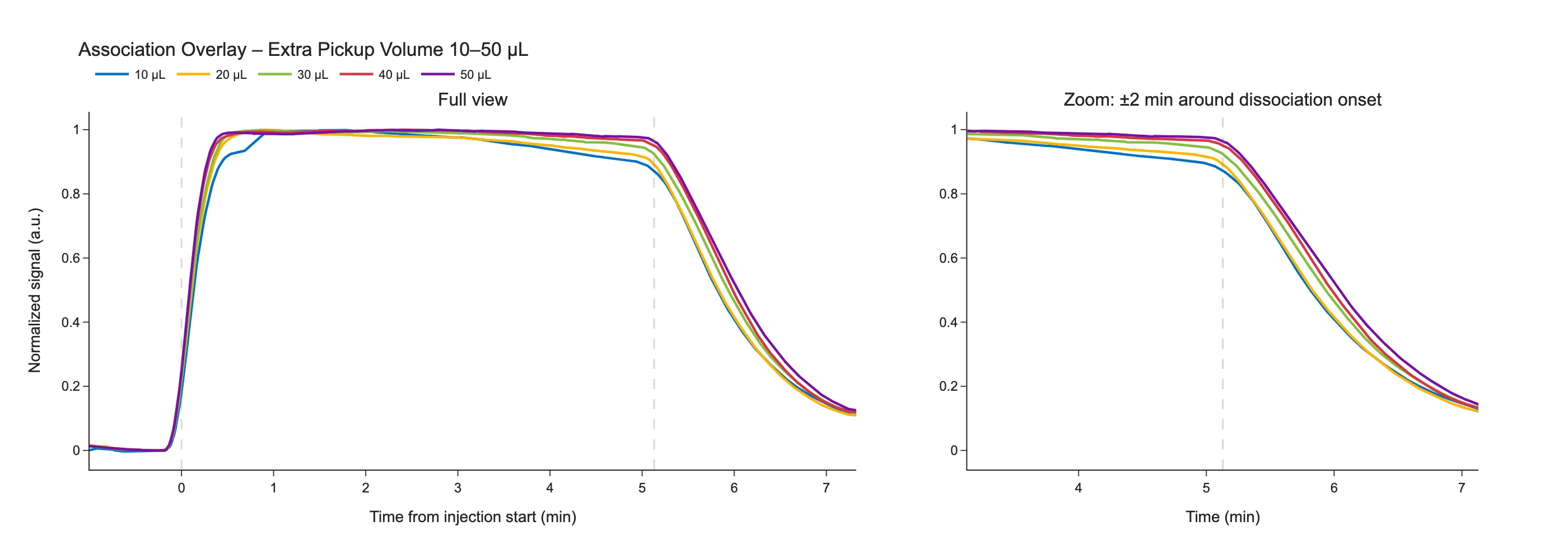
Kinetic Measurements (SCK, MCK, etc.): An extra pickup volume of 30 µL is recommended. This ensures that the sample concentration remains constant throughout the association phase and that kinetic parameters are not distorted by diffusion artifacts. This extra pickup volume is also preset for the kinetic templates in the software, but can be adjusted based on the expected kinetics and flow rates.
Immobilizations: A pickup volume of 30 µL can be used to compensate for tail diffusion effects during immobilization. This is particularly relevant at low flow rates (< 20 µL/min) where the sample spends more time in the tubing and diffusion has a larger impact on the concentration profile.
When to increase: For longer contact times or higher viscosity samples, consider increasing the pickup volume to maintain a uniform concentration at the sensor. Refer to the Inject and Incubate section for guidance on how pickup volume interacts with incubation duration.

The normalized overlay below shows that with an appropriate pickup volume, the diffusion effects from the tubing are effectively compensated. When properly compensated, the association curves from different conditions align and dissociation only starts upon buffer injection, confirming that the analyte concentration at the sensor is constant.

Normalized association phase overlay showing compensated tail diffusion