The MACS Matchmaker is a benchtop instrument for label-free biomolecular interaction analysis. It is built on Focal Molography (FM), an optical biosensing technology that detects molecular binding events in real time and provides quantitative data on binding affinity, kinetics, and specificity. Unlike conventional refractometric sensors, FM is intrinsically insensitive to non-specific adsorption and bulk refractive-index changes, making it well suited to measurements in complex biological matrices such as serum, plasma, and cell lysates.

Principles of Focal Molography

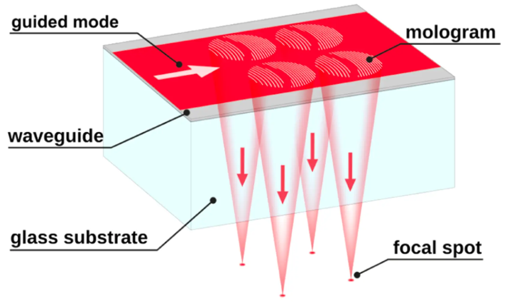
Focal molography translates molecular binding events into optical signals through diffractive interference. The key component is the mologram: a nanostructured diffraction grating covering a 400 × 400 µm area, fabricated directly on the sensor chip by photolithography. The mologram consists of nearly a thousand alternating regions:

• Ridges(~200 nm wide) — functionalized with specific capture molecules (ligands). Analyte binding occurs exclusively here.
• Grooves(~200 nm wide) — passivated with an inert, non-binding coating. They serve as the built-in reference region interdigitated at the nanoscale with every ridge.

A laser beam coupled into the Ta₂O₅dielectric waveguide propagates as a guided mode along the chip, generating an evanescent field that extends approximately 100 nm above the surface — the sensing volume. Light diffracted by mass on the ridges converges constructively at a single focal point, forming a bright focal spot recorded by a camera. The grooves diffract out of phase and cancel destructively at the same point. The MACS Matchmaker chip contains 64 independent molograms arranged in an 8 × 8 grid, each yielding a separate real-time sensorgram. Individual molograms are named SM_RxCy (Single Mologram at Row x, Column y) — for example, SM_R3C4 is the mologram at row 3, column 4.

How molography measures binding: CMD and MD

Every mologram simultaneously produces two independent signals from the same optical readout. They come from different physical properties of the focal spot — its intensity and its position — and carry fundamentally different information.

The sensor: waveguide and mologram

The sensor chip contains a Ta₂O₅dielectric waveguide. A laser is coupled into the waveguide and propagates as a guided mode along the chip, generating an evanescent field extending approximately 100 nm above the surface — the sensing volume in which all binding events are detected. The mologram sits at this surface: a periodic grating with period Λ ≈ 400 nm consisting of nearly a thousand alternating functionalized ridges and passivated grooves.

The diffractometric detection principle

The focal spot responds differently to different surface events, and this is the physical basis of focal molography's selectivity.

Specific analyte binding adds mass to the ridges but not the grooves. This increases the optical contrast between ridges and grooves: more mass on the ridges means more coherent scattering in register with the grating period. The focal spot becomes brighter — its intensity rises. This intensity change is the diffractometric signal, quantified as Coherent Mass Density (CMD).

Non-specific adsorption deposits molecules randomly across the entire surface — on ridges and grooves equally. This does not change the optical contrast between the two regions. The diffracted fields remain balanced so focal spot intensity does not change. Instead, the uniform refractive-index increase shifts the position of the focal spot laterally. Only the positional (refractometric) channel responds; CMD does not.

Bulk refractive-index changes — from temperature fluctuations, buffer exchanges, or high-concentration matrix components such as serum proteins and regeneration reagents — follow the same logic. They affect ridges and grooves identically, shift the focal spot position, and leave its intensity unchanged. CMD is therefore intrinsically blind to these perturbations without any external correction step.

Coherent Mass Density (CMD)

CMD is the primary output of a focal molography measurement. It is derived from the intensityof the focal spot captured by the camera and reported as a surface mass density in units of pg mm⁻². CMD measures only mass bound coherently in spatial register with the mologram grating — exclusively, specific analyte binding on the ridges.

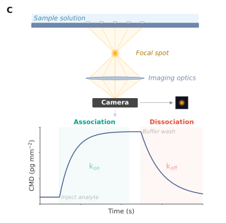
A real-time CMD trace — the sensorgram — reflects the three phases of a binding experiment:

• Baseline: running buffer only; CMD is stable because no analyte is present and there is no coherent mass change.
• Association phase: analyte is injected; CMD rises as analyte binds to the immobilised ligand. The rate of rise is governed by both $k_{\mathrm{on}}$ and the analyte concentration.
• Dissociation phase: buffer replaces the analyte solution; CMD decays as analyte leaves the surface, governed by $k_{\mathrm{off}}$.

Because CMD is insensitive to bulk perturbations, it remains stable across rapid temperature changes. During a continuous 25–45–25 °C temperature ramp, CMD drifts by less than 1 pg mm⁻²— under 0.25 % of a typical protein monolayer (~400 pg mm⁻²). This stability eliminates the lengthy thermal equilibration periods — typically 30–60 minutes per temperature step — required by refractometric instruments, and it enables kinetic measurements directly in complex biological matrices such as human serum without additional correction steps.

Mass Density (MD)

MD is the refractometric channel of the same instrument, derived from the positionof the focal spot. When the local refractive index at the sensor surface changes — for any reason — the focal spot shifts laterally. The magnitude of this shift is converted to a surface mass density, also reported in pg mm⁻².

MD is physically analogous to the signal from a surface plasmon resonance (SPR) instrument: it responds to all refractive-index changes regardless of their origin — specific binding, non-specific adsorption, temperature drift, and buffer composition changes alike. A typical protein monolayer corresponds to approximately 2000–4000 pg mm⁻²in MD, compared to ~400 pg mm⁻² in CMD.

The sensitivity of MD to bulk effects is also its principal limitation in complex media. During a 20 °C temperature ramp, MD shows an apparent signal excursion of several thousand pg mm⁻². Even after active referencing by pairwise sensor subtraction, residual drift spans ±2000 pg mm⁻²— comparable to a full protein monolayer. In 50 % human serum, matrix components overwhelm the MD trace, and regeneration pulses produce spikes of up to 15 000 pg mm⁻², largely masking any specific binding response.

MD is nonetheless useful as a diagnostic channel. Because it captures every refractive-index event at the surface, it can confirm sample delivery, detect air bubbles, identify gross surface fouling, and flag thermal instability — all from the same measurement as CMD.

Sub-micron self-referencing vs. a separate reference channel

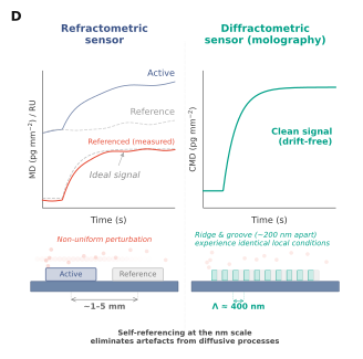
In conventional refractometric biosensors such as SPR, non-specific signals are subtracted using a reference spot located millimetres away from the active spot on the same chip. This approach assumes both spots experience identical perturbations — an assumption that breaks down for spatially non-uniform events. Diffusing serum components, localised temperature gradients, and regeneration pulses that arrive at slightly different times at the two spots all produce residual artefacts that can be comparable in magnitude to the binding response itself.

In focal molography, referencing occurs at the 200 nm scale: every ridge is immediately flanked by a groove separated by the width of a single mologram period. Both experience identical local conditions — the same evanescent field, the same flow, the same temperature — because they are separated by far less than the diffusion length of any perturbation. Non-specific contributions cancel completely and automatically, with no spatially separated reference required.

CMD and MD at a glance

Rejecting non-specific binding

Because CMD reports only the coherent mass difference between ridges and grooves, molecules that adsorb uniformly across the whole surface are invisible to it. In crude media the surface chemistry of ridges and grooves is deliberately matched — backfilling — so that high-abundance matrix proteins bind both regions equally and their contribution cancels, leaving only the specific analyte signal.

Backfilling is the key to measuring in serum, plasma, and lysate. Backfilling and NSB suppression covers what it is, how to choose and tune the backfill probe, and how to verify a matched chip.

Mass Transport

Analyte must diffuse from the bulk solution across an unstirred boundary layer before it can bind. When the surface binds faster than diffusion can replenish analyte ($k_t \lesssim k_{\mathrm{on}}\,[\text{ligand}]$), the measurement becomes diffusion-limited and the fitted k_on underestimates the true on-rate. Raising the flow rate and lowering the ligand density push the assay back into the reaction-limited regime.

For the full treatment — symptoms, mitigations, and an interactive simulator — see Mass transport limitation in Biomolecular Interaction Analysis; see also Recommended Flow Parameters and Ligand surface density.

Ligand surface density

The amount of ligand immobilised on the ridges sets the maximum signal $R_{\max}$, but density also strongly shapes the apparent kinetics — so more is not better.

• Too high. A dense surface consumes analyte faster than diffusion can supply it, producing mass-transport limitation and an underestimated $k_{\mathrm{on}}$. Dissociated analyte is also more likely to rebind a neighbouring site before leaving, which flattens the dissociation phase and underestimates $k_{\mathrm{off}}$. For multivalent analytes, high density promotes avidity and steric crowding.
• Too low. The signal approaches the noise floor, giving poor signal-to-noise and unstable fits.

For clean kinetics, use the lowest density that still gives an adequate signal — a low-$R_{\max}$, transport- and rebinding-free regime. On DDI chips, density is tuned by mixing the capture and adaptor strands, by shortening the immobilisation, or with a stop condition. See Ligand Density vs. Mass Transport Trade-Off and R_max Estimation.

Limit of detection and sensitivity

The limit of detection (LOD) is the lowest analyte concentration that can be reliably distinguished from a blank — conventionally the concentration whose signal exceeds the blank by $3\sigma$, where $\sigma$ is the standard deviation of the blank response.

On a refractometric sensor in a crude matrix, non-specific binding raises and broadens the blank, so the LOD is dominated by NSB rather than by the instrument. Focal molography removes this term: because coherent NSB is rejected by affinity-matched backfilling, the blank stays flat even in undiluted serum or plasma. The detection floor is then set by instrumental and photon noise and by mologram-to-mologram reproducibility — not by the sample. In practice this means the LOD in undiluted plasma is comparable to the LOD in buffer (of the order of 10² pM for a short assay, improving with longer association), where a refractometric assay would require dilution, washing, and proofreading steps.

Levers that improve the LOD: average more replicate molograms (random noise falls as $1/\sqrt{N}$), extend the association phase to accumulate more bound mass, and run a sufficient number of blanks (≥ 5) to characterise $\sigma$ well. The guided LOD workflow is described under Evaluations and the LOD phase template under Assay Phases.

For term definitions, see the Glossary.