MACS Matchmaker
The MACS Matchmaker produces time-resolved coherent mass density (CMD) traces. This page covers both the tool — how to work in Insights after a run finishes — and the interpretation — which binding model to use, how to validate the fit, and how to report results. If you are new to kinetic analysis, start with Biomolecular Interaction Analysis first.
Part 1 — Working in Insights
The software reference for post-measurement analysis: project-level workflows, the Data Clean Up dialog, Report Points, per-phase Evaluations (SCK, MCK, LOD), and the Fit Timetraces tool.
Insights
Everything after measurement is stored on the Insights page. Plot measurements, clean them up, save the cleaned data, and use them for evaluations. Project-level goal cards group related workflows (below) by evaluation type; per-phase evaluations (SCK, MCK, LOD — see further down this page) run on a single measurement phase.
Workflows
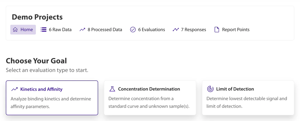
The project home groups available evaluation goals into Kinetics and Affinity, Concentration Determination, and Limit of Detection. Open Kinetics and Affinity to start a guided study setup, name and tag the study, choose between Binding Kinetics, Equilibrium Analysis, and DEL Evaluation, and then continue through the setup directly on the page. Open Limit of Detection to enter the evaluation name, tags, and description, select eligible raw data, processed data, or an existing evaluation, configure the response and fit parameters, and review the key settings before starting the evaluation. Binding Kinetics studies ask whether to run Determine Kinetics, SCK, or MCK before data selection. Every guided evaluation accepts the compatible source types shown in its Data step. While compatibility is checked, each row shows a spinner in a fixed-size selection control; unsuitable rows remain visible but disabled, and their selection controls show the validator message that explains which requirement the data does not meet. Raw data can also be added to the project directly from the Data step. Data-selection tables reserve their widest column for the source name and omit the description column so long names remain identifiable. The standard stepper shows Goal, Data, Parameters, and Review. Equilibrium Analysis shows Goal, Data, Cleanup, Parameters, and Review. Determine Kinetics shows Goal, Data, Cleanup, Parameters, Fitting, and Review so cleanup always comes before the fitting setup. Step numbers stay aligned when labels wrap on a narrow screen. The footer groups Cancel, Back, Next, Run, or Save actions on the left. Once anything has been entered, Cancel asks for confirmation before it leaves the workflow, because leaving discards the setup. The same confirmation appears when the workflow is left in any other way, such as the browser back button or a reload, while an untouched workflow is left without a question. Review summarizes the key setup values, including the names of cleanup actions inherited from selected data and applied by the workflow. It displays the first three action names and an ellipsis when more are present; select the summary to show or hide the complete list. The final Run action starts and saves every evaluation. Concentration Determination opens a guided workflow for naming the study, selecting calibration data and unknown data together, cleaning each selected input, configuring prediction parameters, previewing the generated plots, and optionally saving the evaluation. Its steps are Details, Data, Cleanup, Parameters, Fitting, and Review. A calibration measurement with an Unknown Concentration phase selects itself as the unknown automatically.
Re-evaluating an evaluation opens the same guided setup it was built in, with its data, parameters, description and tags filled in and its name carrying the next version: re-evaluating Sample proposes Sample (Version 2), and re-evaluating that proposes Sample (Version 3). A setup opened this way, or from a Use for … Evaluation button on processed data, starts past the steps its link has already answered: at Cleanup for Determine Kinetics, at Fitting for Concentration Determination, and at Parameters for every other evaluation. The earlier steps stay open in the stepper. Concentration Determination fills its calibration and its unknown role separately, each from the raw data that role ran on. Determine Kinetics also restores the fits you accepted and rejected by hand, together with the fit rejection strictness, so its fitting step opens where you left it. What the strictness decided is not carried over but worked out again from the new fits, so a fit rejected automatically comes back as an automatic rejection you can still overrule, and one that no longer converges is marked invalid. Selecting an evaluation as the data source in a Data step contributes its data only, together with the data selection and cleanup actions stored with it; the parameters stay at the defaults for that data. The Evaluations list in a Data step offers only evaluations of the kind being set up, so the data it hands over is data that kind of evaluation has already run on.
Common settings stay visible in the main parameter cards. Less frequently changed settings are collected in Advanced Parametersand collapsed initially. Equilibrium Analysis configures interactive cleanup actions and automatic cleanup in its Cleanup step. SCK and MCK keep Auto Data Cleanup and the actions it controls together in a dedicated Data Cleanup card in Parameters. Parameter labels include the scientific unit or state that a value is a fraction or dimensionless. Evaluation plots are generated automatically, so the guided workflows do not require a separate plot checkbox.
Binding Kinetics modes
- Determine Kinetics: clean and fit one dataset interactively to estimate kinetic rate constants and affinity. Use Cleanup to review cleanup actions and Fitting to inspect and accept or reject fits. The info button at the right of Model Summary opens the interactive simulator for the selected binding model.
- SCK (Single-Cycle Kinetics): inject increasing concentrations in one cycle without regeneration between injections. This uses less sample and finishes faster.
- MCK (Multi-Cycle Kinetics): measure one concentration per cycle and regenerate between cycles for independent binding cycles.
The Kinetics and Affinity wizard includes an Evaluation Assistant when the shared assistant service is enabled. It starts with the current goal, step, and data selection so you can ask about model choice, data requirements, cleanup, fit acceptance, or review. Its answers use the same grounded product and science documentation as the Documentation Assistant.
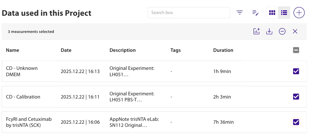
Use the Project Overview metrics to jump from the home page to Raw Data, Process Data, Responses, Evaluations, or Report Points. To assign measurements to the project, open Raw Data and use the add (+) action there. Data steps that accept measurements, including Kinetics and Affinity and Limit of Detection, also offer an Add Raw Data to Project action.
Raw Data plots show all signal molograms by default for multi-channel flow chambers and multiplexed measurements. A 1-plex Sirius 8×8 measurement made with the single flow chamber starts with the inner signal molograms selected; the mologram picker can change either selection.
DEL Evaluation
Workflow for DNA-encoded library (DEL) hit validation. The assay immobilizes DNA-labeled compounds onto multiplexing groups on the sensors and then runs a single-cycle kinetics titration against the analyte of interest. Ligand and individual-sensor thresholds filter weak response-to-immobilization ratios before fitting. Reduced chi-squared thresholds control model selection and fit acceptance.
Configuration
| Setting | Scientific and operational meaning | Default |
|---|---|---|
| Threshold Ligand | A dimensionless fraction from 0 to 1. For each ligand, the evaluation takes the median response divided by immobilization and compares it with the strongest median in the selected data. The ligand continues to fitting only when its median is at least this fraction of that reference. A higher value is stricter and rejects more weakly responding ligands. | 0.2 |
| Threshold Individual Sensor | A dimensionless fraction from 0 to 1. Each sensor's response-to-immobilization ratio is compared with the largest ratio in the selected data. The sensor continues to fitting only when it reaches at least this fraction of the maximum. A higher value is stricter and removes more low-response sensors. | 0.1 |
| Auto Data Cleanup | Runs the selected blank-subtraction actions before filtering and fitting. Turn it off to fit the selected traces without these automatic corrections. An action leaves the data unchanged when its required blank structure is not present. The master setting and all available blank-subtraction choices are kept together in the same outlined group. | Enabled |
| Subtract blank phase | When Auto Data Cleanup is enabled, finds phases with matching single-cycle injection structure, treats the phase with the lowest total response as the blank, and subtracts it from the phase with the highest response. At least two compatible phases are required. | Selected |
| Subtract blank injection group | When Auto Data Cleanup is enabled, uses the first blank injection group in each single-cycle sequence as the reference. It subtracts that group from later target groups whose dissociation duration is no more than 10% longer than the blank, removes the blank group, and reconnects the processed trace continuously. | Selected |
| Subtract blank molograms | When Auto Data Cleanup is enabled, identifies sensors without an immobilized ligand, averages their traces, and subtracts the average blank signal from every ligand-bearing sensor. Blank sensors are removed from the processed sequence. | Selected |
| Reduced Chi-Squared Stickiness Threshold | A dimensionless threshold in the collapsed Advanced Parameters section. The evaluation first estimates off-rates at the highest concentration and takes the median reduced χ² across sensors. A median above this threshold classifies the ligand as sticky and selects the partially non-dissociative Langmuir 1:1 model. A lower threshold classifies more ligands as sticky. | 5 × 10⁻⁴ |
| Reduced Chi-Squared Fit Quality Threshold | A dimensionless threshold in the collapsed Advanced Parameters section. A sensor fit is rejected when its reduced χ² is at or above this value. A lower value applies a stricter fit-quality requirement; a higher value accepts more fits. | 1 × 10⁻² |
| Automatic plot generation | Every DEL evaluation generates its report plots without a separate checkbox. Available outputs include response and immobilization overviews, sequence and compound time traces, and per-sensor fit, fit-overview, and off-rate plots. A plot is omitted when its required data are unavailable or that plot cannot be produced. | Always enabled |
Determine Kinetics
Guided kinetic analysis for binding experiments. Select raw, processed, or previously evaluated data, configure fitting parameters, clean up sensors if needed, inspect model fits, review the setup, and run the evaluation report. Determine Kinetics reviews cleanup actions inside its Cleanup step instead of using the SCK/MCK auto-cleanup option. Cleanup actions configured there remain applied through Fitting and final report creation. Use Save as processed data only when the cleaned input should also be reusable outside the wizard. Its fitting view distinguishes a fit that did not converge from a converged fit with poor quality. Adjusting fit rejection strictness updates automatic decisions; manually accepted fits are preserved. Select the mologram name at the top of a fit preview to inspect it in Single Mologram. Grids with more than four previews hide the repeated axes, and a failed fit stays gray in the grid; its failure message appears after opening the individual plot. Fit-subtraction cleanup actions apply only to molograms in the current data selection, so they remain usable when the selection changes. The Review card summarizes the selected data, model, initial parameters, cleanup, and fit settings before the evaluation runs. Kinetic parameters identify kon in M−1 s−1, koff in s−1, normalized Rmax as dimensionless, and the normalized mass-transport constant kt in M−1 s−1. When Fitting opens, the view defaults to Single Compound when more than one compound is present, otherwise Single Mologram, and the Parameters tab is selected first. If an evaluation fails, its selected data and cleanup actions are automatically saved as processed data so the work can be recovered.
Equilibrium Analysis
Fit equilibrium endpoint responses across analyte concentrations to estimate affinity without kinetic rate constants. Its Cleanup step previews the selected response and lets you add, edit, or remove cleanup actions before configuring the fit. Actions configured there are carried into the evaluation; Save as processed data is only needed when the cleaned input should also be reusable elsewhere. The Automatic Cleanup tab controls the equilibrium-specific offset removal, supported blank-subtraction actions, and optional immobilization normalization that run after the interactive actions.
Concentration Determination
Estimate the concentration of an unknown sample from its endpoint response, using a previously measured standard curve. Provide a reference titration that establishes the curve and one or more unknown samples measured under matched conditions; the system inverts a 4PL, zero-baseline 3PL, or scaled through-origin cubic model per sensor and combines per-dilution back-calculated values into one overall estimate. Logistic models receive high-concentration plateau assessment; the non-saturating cubic model does not. Predictions inside the final fitted calibration range use interpolation. Responses outside the fitted boundary have no predicted concentration and zero effective weight; they are not extrapolated or endpoint-clamped. Each sensor fit is plotted only over its retained-standard interval. The Data step contains both calibration and unknown selections, and Cleanup lets you preview and edit every input independently. Final concentration normalization and sensor aggregation are configured once in Parameters, together with automatic outlier removal and an optional known concentration in Advanced Parameters; Review blocks double normalization and lists cleanup actions separately. Fitting provides model selection, the calibration curve, concentration boxplot, per-injection sensor tables, and manual calibration and unknown exclusions. The final Review step lists the setup, numeric result summary, and warnings. Completed evaluations can be re-evaluated from the Evaluations table; the prior evaluation is preselected for both data roles, and its fitting settings and exact calibration and prediction exclusions are restored. See Concentration Prediction for data requirements, configuration, and how the combined estimate is computed.
Limit of Detection
Estimate the smallest reliably detectable concentration from a titration series and blank measurements. Select eligible raw data, processed data, or an existing evaluation, or add raw data to the project without leaving the Data step. Auto Data Cleanup and its available actions are grouped in the LOD Fit card, percentile fields are entered as percentages, and Save Intermediate Fits is in the collapsed Advanced Parameters section.
Data Clean Up
The CLEAN UP DATA dialog organizes actions into category cards. Choose a category, then choose an action card whose description matches the result you need. The navigation header shows the current category and action; select an earlier item in the header to return to that overview. You see the effect of each action directly in the plot on the left. Configure the action and select Apply. Actions can be deleted, but later actions that depend on earlier ones will be deleted too if you remove the earlier step. In the Determine Kinetics wizard, use Save as processed data to keep the current result without leaving the workflow. To leave molograms out of the evaluation, deselect them in Update data selection (the tune button above the plot) instead of adding a cleanup action.
Cleanup Actions Reference
Each row below corresponds to one action category in the dialog, keyed by the same anchor for deep linking.
| Category | Actions |
|---|---|
| Cut Out |
|
| Edit |
|
| Offset |
|
| Normalization |
|
| Smoothing |
|
| Blank Subtraction |
|
| Zero-Crossing | Zero-crossings occur when the coherent mass on the grooves exceeds that on the ridges, causing the diffractometric signal to pass through zero and invert. They typically appear during high-concentration injections in complex media when backfilling is suboptimal.
|
| Data |
|
| Injection Groups | Use Split Into Injection Groups to organize injections into groups before performing group-level operations. Useful for MCK and titration experiments with repeating injection patterns. Some blanking actions (like Subtract blank injection group) require grouped injections. |
Report Points
A report point is a statistical summary of the signal over a short time window. Report points can be created manually by clicking into the plot, selecting a duration, and specifying a description, or generated automatically from the injection sequence (see Automatic Report Points below). They can then be analyzed on the Report Points page in Insights. For each report point, multiple values are calculated and a summary over all sensors is displayed in the first row. A dropdown reveals metadata and individual sensor values. Report points can be exported as CSV for further processing.

Configure Report Points
The Configure Report Points dialog previews the report points for a measurement before you rely on them. Open it from a plot on the Perform page, or from the More actions menu of any entry in a project's Processed Datatable. When opened from processed data, the entry's clean-up actions are applied first, so the plot (with report-point markers), the Report Points Table, and the export all reflect the processed (cleaned) data. In that mode the phase comes from the processed-data selection and the plot uses the marker-supported consensus view; holograms, injection-type settings, and the back-fill threshold remain editable.
CSV export
The dialog-level Export CSV button exports all sensor valuesalongside the consensus summary: the file contains one row per report point and sensor, each with its own mean, median, standard deviation, maximum, minimum, and slope, plus the report point's consensus (over-all-sensors) median, mean, and slope repeated on every row. Every row also carries the measurement name, sensor name, ligand name, the report-point timestamp, and the selectedtime window (s). The per-sensor mean is the arithmetic mean of that sensor's values inside this window; the consensus mean is then the mean of the per-sensor means. This makes it possible to trace every exported mean back to the interval used for its calculation while the consensus median remains available.
The Report Points Table also includes a Show Details action for each row. It opens a per-report-point view with a sensor heatmap, a sensor-value boxplot, and a CSV export containing only that report point's per-sensor rows.
Save to project
Automatically detected report points can be saved so they persist and appear on the Report Points page. Click the save icon in the Report Points Table header to reveal a checkbox on each savable row, select one or more report points, and click Save to Project. When the dialog is opened inside a project the report points are saved to that project directly; otherwise you pick the target project from a dropdown. Manually created report points and automatically detected points that were saved previously are already stored and cannot be re-saved. If part of a multi-point save fails, only the failed report points remain selected for retry.
Report Point Calculations
For each report point, the system evaluates the selected report-point time window (for example the configured 5-second window near an injection end). It first computes a consensus trace (also called median trace) by taking the median value across all sensors at each time point — a robust central estimate that is less affected by outliers. All report-point values are then derived from the consensus trace and the individual sensor traces:
- Value: the consensus trace value at the report-point timestamp.
- Slope: the mean of slopes computed across all individual sensor traces within the report-point time window (linear regression per sensor; arithmetic mean across sensors).
- Delta:the difference between this report point's value and the previous report point's value in the sequence.
Automatic Report Points
When viewing a measurement with injections, report points can be generated automatically based on injection type:
| Type | Placed on | What it captures |
|---|---|---|
| Capture Level | Immobilization injections | Amount of ligand captured on the surface. |
| Binding Start | Association injections | Placed at the minimum value in the 20-second window before the injection starts — the baseline reference. |
| Binding | Association injections | Placed near the injection end. |
| Stability Point | Dissociation injections | Placed at the first timestamp where the signal drops by 5% relative to the previous Binding Start (or the baseline if no Binding Start exists) — marks the onset of dissociation. |
Evaluations
After selecting a phase of your measurement, run evaluations and review the results in the relevant evaluation views under Insights. Each phase only supports the evaluation types that are valid for that experiment design.

Response Plot Units
Evaluation plots label and scale the response axis from the response quantity. Normalized responses are dimensionless and are shown as normalized (a.u.). Coherent mass density is shown in pg/mm² using one conversion from its base unit to the display unit. Measured points and fitted curves therefore use the same scale.
Evaluation Result Findings
Completed SCK, MCK, Determine Kinetics, DEL, and Concentration Determination evaluations display a compact, result-specific findings panel automatically. A stateless findings service reads the evidence saved by the evaluation. It does not invoke an LLM, rerun the evaluation, or parse a generated report.
SCK, MCK, Determine Kinetics, and DEL use the same compact report: accepted and rejected counts appear below the findings title, outcome rows state the conclusions, and bounded exceptions or recommended actions are available under Technical details. The saved observations include:
- Result summary: how many fits or ligands were accepted and rejected. Only accepted results are used in the conclusions.
- Fit quality:a short ligand-level conclusion naming the model and confirming that accepted results passed the evaluation's fit-quality gate. If koff was estimated from a dissociation segment and held fixed in the global fit, the finding still reports a successful fit while qualifying koff and KD. Clean SCK/MCK design reports do not repeat this row.
- Main binding results: for multiplex chips, which ligands have similar on/off-rate behavior. A ligand with only one accepted sensor or an unresolved off-rate is left unclassified.
For an SCK or MCK evaluation using the strict Langmuir 1:1 model, the evaluation checks every accepted fit against the concentration series, programmed association and wash durations and final dissociation recorded for that result, plus its measured sampling interval. Autosampler pickup gaps may extend the plotted trace intervals but do not change the programmed durations checked here. When every accepted fit forms an exact design request, the findings cover equilibrium suitability, 1:1 fit design, association timing, dissociation timing, and any fitted rate outside the measurable range. This deterministic guidance replaces the generic concentration and dissociation suggestions instead of duplicating them. If any accepted fit is not exactly representable, the complete design section is omitted and the generic concentration and plateau cautions are used.
Concentration Determination uses the same deterministic findings panel with concentration-specific evidence. Its summary reports how many unknown/dilution prediction groups were attempted and contributed to the combined estimate. Estimates inside the final fitted calibration interval use interpolation. A response outside the fitted values at those retained-standard boundaries has no predicted concentration and zero effective weight; it is never extrapolated or endpoint-clamped. Each sensor fit is plotted only over its retained-standard interval. When relevant, the range finding reports below-range, above-range, and unavailable sensor counts with bounded per-group detail, including each affected sensor's measured response and status. Fitting contains the calibration curve, boxplot, and selectable per-injection tables; Review contains the study and numeric result summaries plus warnings. The completed result uses this findings panel as its single diagnostic summary instead of repeating those workflow warning alerts. For logistic models, a separate calibration finding warns when any assessable curve reaches less than 90% of its fitted high-concentration plateau or a curve cannot be assessed; it reports the affected curve count and, when a curve is assessable, median coverage, threshold, and the highest retained standard. This plateau assessment does not apply to the non-saturating cubic model.
A separate dilution-response-compression check examines the three highest sample fractions only when they span at least 4× in dilution factor. It normalizes each sensor's responses to the fitted response interval between the lowest and highest retained calibration standards. A sensor is compressed when all three responses stay at or above the 75% calibrated response position and span no more than 15% of that interval; the warning appears when at least four sensors are assessable and at least half are compressed. This is an advisory warning for possible response saturation or dilution-series inconsistency and does not change exclusions or weights.
An older result that does not contain the saved evidence shows an explanation that the evaluation must be re-run or re-evaluated. Missing saved evidence does not mean that every ligand or prediction was rejected.
For supported kinetic and DEL evaluations, Ask appears with an AI sparkle icon in the findings header when the shared LLM API is configured and opens a right-side conversation. The findings remain visible without an LLM; only Ask is omitted. Concentration Determination displays deterministic findings without offering Ask. The assistant always receives the same bounded findings shown in the panel and a catalog of the names in this result. When a question needs more, it requests fit details, rejection evidence, or derived responses, and those lookups run on the Hub against this evaluation only. Every returned fit row is marked accepted or rejected; rejected rows explain exclusions only. The tools are read-only and cannot change stored data. With exact rate, timing, concentration, mode, and sampling inputs, the assistant can also run the same deterministic SCK/MCK design check as the phase editor. Missing inputs are requested rather than replaced with defaults. That what-if uses the same finding structure, carries no plot arrays, does not replace the saved evaluation evidence, and cannot apply suggested experiment changes. Artifact file contents are not treated as inspected.
Each conversation belongs to the person who started it and to one evaluation. A question and its answer are saved together once the answer finishes, so an interrupted answer leaves the conversation unchanged.
Exact values, plots, residuals, and sensor tables remain in the evaluation result. Findings use count-first outcomes and keep bounded exception evidence under Technical details; they contain no plot data. The assistant receives the same compact records. Multiplex groupings describe this measurement only; they do not establish biological classes.
DEL and Concentration Determination create this evidence from the same processed result used to build their saved artifacts. If a future conclusion needs a value that is not persisted, that deterministic calculation is added to the evaluation first. The findings service only selects, compares, and explains stored evidence.
SCK (Single Cycle Kinetics) Evaluation
Add your data to a project and create a processed-data element with the SCK phase. Click USE FOR SCK EVALUATION to open the guided setup on its Parameters step, with that processed data already selected and named after it, choose the model for fitting, and run. Results appear in the evaluation view. If you have cleaned up the data manually, do not use the auto-cleanup button — your changes will be overwritten. Every optimizer-converged SCK fit remains in the saved results and standard fit artifacts. SCK does not apply a final fit-rejection strictness filter. The result view adds a tagged Rejected fits artifact only when fitting does not produce a usable result for a mologram; it can be shown or hidden with Filter by tags. Slow-dissociation results remain successful and add a warning that recommends a longer dissociation phase. For existing data, correct only visible drift or baseline offsets and exclude injections with spikes or other artifacts; cleanup cannot compensate for a dissociation phase that is too short. Auto Data Cleanup and its available actions are kept together in an outlined group, while initialization and drift correction are in the collapsed Advanced Parameters section. Manual initial-parameter fields identify kon in M−1 s−1, koff in s−1, normalized Rmax as dimensionless, and the normalized mass-transport constant kt in M−1 s−1.
For the physics of each model, see the Binding Models table below or use the info button at the right of Model Summary to open the simulator for the selected model.
Slow dissociation warnings
SCK assigns each sensor fit one of three classifications:
- Complete kinetics — both kon and koff are quantifiable. The result includes kon, koff, and KD.
- Association rate only — koffis below the dissociation phase's detection limit. The fit remains successful: its fitted curves and kon remain available, with the fitted uncertainty interval when it can be calculated. The result reports koff as
< detection limitand KD as unavailable. - Unusable — fitting did not produce a successful result for the mologram. It is excluded from saved kinetic results and listed in Rejected fits with the failure reason.
The koff detection limit uses a fixed 5% criterion. The longest fitted dissociation must support at least a 5% signal decrease for koff to be quantifiable:
k_off detection limit = −ln(0.95) / dissociation durationA converged SCK fit is not passed through a final fit-quality or strictness rejection filter. A low koff is therefore warning-only, and no additional option is required. The result page keeps the standard fit artifacts and adds a koff warning with the observed decay and the recommended longer dissociation phase.
MCK (Multi Cycle Kinetics) Evaluation
Similar to SCK but intermediate regenerations are performed before each cycle. Choose the model to fit and run.
Equilibrium Evaluation
Equilibrium evaluation extracts a steady-state dissociation constant (KD) from the plateau response at each analyte concentration. It complements SCK/MCK kinetic fitting: kinetics give kon and koff from the time-course, equilibrium gives KD from the height of the plateau. The two should agree when binding is well-behaved 1:1 — disagreement is diagnostic. See BIA → Equilibrium for the underlying physics.
When to choose Equilibrium over kinetic analysis
- You only need affinity (KD), not residence time or rate constants.
- Kinetic fitting is unstable on your data — for example mass-transport limited association, complex curve shapes, or surface decay.
- You want a robust cross-check against a kinetic KD obtained from the same trace.
Data requirements
- A single phase with at least two ASSOCIATION injections of the same analyte at different concentrations, or two or more grouped traces with one association each. SCK-format and MCK-format data are both accepted.
- A valid concentration must be set on each association. Injections without concentrations are silently excluded; if fewer than two remain, the evaluation aborts with an error.
- For a stable 4PL fit, aim for at least six concentrations spanning two decades and bracketing the expected KD (≥2 below, ≥2 above). Fits with fewer points succeed numerically but become unreliable.
- A BASELINE injection before each association gives the preprocessor a clean reference for offset removal. Without one the system falls back to a derived window and emits a warning.
How to run it
- Add the measurement to a project, or open the evaluation wizard and use Add Raw Data to Project from its Data step.
- From the project home, open Kinetics and Affinity, then chooseEquilibrium Analysis.
- Select eligible raw data, processed data, or an existing evaluation's inputs. Configure cleanup actions in Cleanup, choose the fitting settings in Parameters, review the setup, and choose Run.
- Results appear in the evaluation view: per-sensor 4PL fits, aggregate KD with confidence interval, and exportable plots.
Configuration
| Parameter | Purpose |
|---|---|
| Model | Currently fixed to Four Parametric Logistic Regression (4PL). Fits plateau response vs. concentration and reports KD, Hill slope, and the bottom/top asymptotes. |
| Fit Equilibrium | When enabled, fits an exponential saturation curve to each association and uses the extrapolated steady-state value (req). Use this when association windows are too short to actually reach the plateau. When disabled (default), the response is the mean signal over the percentile range below. |
| Response / Fitting Interval | Dimensionless fractional window from 0 to 1 used for response extraction. Default [0.9, 0.95] averages the 90th to 95th percentile of the association, which approximates equilibrium for well-saturated traces. Defaults flip to [0.0, 1.0] when Fit Equilibriumis on so the whole association is used for the saturation fit. Both values must lie in the dimensionless [0, 1] interval with start < end. |
| Cleanup Actions | The Cleanup step previews the selected response and lets you add, edit, or remove actions before running the analysis. These actions are stored with the evaluation input. For a reused evaluation with multiple data inputs, the editor updates the first input while retaining the remaining inputs and their existing actions. Use Save as processed data only to make the cleaned input reusable outside the wizard. |
| Auto Data Cleanup | Configured in the Cleanup step's Automatic Cleanup tab. It runs equilibrium-specific offset removal, optional blank subtraction (phase, injection group, molograms), and optional immobilization normalization after the interactive cleanup actions and before fitting. Disable it for custom or mixed datasets where those automatic operations are not appropriate. |
| Subtract Blank Phase / Injection Group / Molograms | Three independent blank-subtraction strategies. Availability depends on the data layout; only options the validator can apply are shown. |
| Normalize to Immobilization | Divides each sensor's response by its immobilization level so sensors with different ligand densities can be compared on a common scale. Enabled by default. |
| Save Intermediate Fits | Stores the per-injection exponential saturation fits when Fit Equilibrium is on, so each association curve can be inspected. This less frequently changed option is in the collapsedAdvanced Parameters section. |
How KD is calculated
For each sensor, the plateau responses at each concentration are fit with the four-parameter logistic model:
y(x) = (min − max) / (1 + (x / POI)^slope) + maxPOI(point of inflection) — reported as KD: the concentration at half-maximum response.min,max— bottom and top asymptotes.slope— Hill slope; equals 1 for a true 1:1 Langmuir isotherm.
If the concentration range does not bracket the inflection, the fitter constrains POI to the sampled range. The returned KD is then a boundary value, not a measurement — extend the range and re-run.
Results
- KD, Hill slope, and min/max asymptote per sensor.
- Aggregate KD reported as the median across sensors with a 95% confidence interval.
- Dose-response plots (per-sensor and overlay), normalized binding- trace plots per ligand, per-sensor timetrace HTML plots, PDF report, and CSV exports of the fitted parameters.
Cross-check against kinetic KD
The same trace can be evaluated both ways. Agreement within a factor of two on the same data is a strong validation of the binding model. Disagreement is informative:
| Symptom | Likely cause | What to do |
|---|---|---|
| KD, kinetic > KD, equilibrium | Mass transport limits apparent kon. | Increase flow rate or lower ligand density; trust the equilibrium value. |
| KD, equilibrium > KD, kinetic | Association too short — plateau not reached. | Extend association time, or enable Fit Equilibrium. |
| Hill slope ≠ 1 | Cooperativity, heterogeneous ligand, or avidity. | Switch to a richer kinetic model (Heterogeneous Ligand, Bivalent). |
| KD sits at the edge of the concentration range | Range does not bracket KD. | Add concentrations below or above and re-run. |
Troubleshooting
- “Insufficient data for equilibrium fitting” — fewer than two ASSOCIATION injections carried valid concentrations. Check that every association has its analyte concentration set.
- “No successful equilibrium fits” — the 4PL did not converge on any sensor. Likely causes: response amplitude near noise, non-monotonic dose-response, or all concentrations on a single asymptote.
- “Baseline inferred from association” — no BASELINE injection was found before an association; the preprocessor used the early portion of the association as a substitute. Add a short baseline before each association to eliminate the warning.
- KD looks unreasonably round (exactly the highest or lowest concentration) — the fitter has clipped the inflection to the sampled range. Extend the concentration range.
LOD (Limit of Detection) Evaluation
The LOD evaluation determines the lowest concentration of analyte that can be reliably detected above the noise level. It runs on Titration Series and Limit of Detection phase types. For the recommended experimental setup (flows, blanks, injection volumes), see Assay Setup → Limit of Detection.
From the project home, open Limit of Detection and follow the guided setup: enter the evaluation name, tags, and description, select eligible raw data, processed data, or an existing evaluation, configure the parameters below, and review the key settings before running the evaluation. Use Add Raw Data to Project to add a measurement without leaving the Data step. Auto Data Cleanup and its available actions are grouped in the main LOD Fit card; Save Intermediate Fits is in the collapsed Advanced Parameters section. Review lists cleanup actions already present in the selected data together with the automatic actions configured for the run, showing the first three names followed by an ellipsis when necessary. Select that summary to expand or collapse the complete list.
Configuration
| Parameter | Purpose |
|---|---|
| Number of Concentrations in Fit | Number of lowest-concentration points used for the linear regression (default 4, range 2–20). |
| Response Mode | Endpoint uses the equilibrium signal at the end of each injection (standard LOD approach). Initial Slope uses the initial binding rate from the beginning of each injection (fits a linear regression per injection). |
| Endpoint Start / End Percentile (%) | Percentage positions from 0% to 100% that define the endpoint response window. The end must be at least 1 percentage point after the start. |
| Baseline Start / Slope End Percentile (%) | Percentage positions used in Initial Slope mode. Baseline start must be no later than 30%, and the slope range must span at least 5 percentage points. |
| Fix Origin Through Median of Blanks | Forces the linear fit to pass through the median response of blank measurements — improves accuracy at low concentrations (enabled by default). |
| Auto Data Cleanup | Baseline offset removal and titration-sequence grouping always run before LOD analysis. Auto Data Cleanup controls the selected blank phase, blank injection-group, and blank-mologram subtraction actions. The available blank actions depend on the selected data. |
| Save Intermediate Fits | Saves individual fitting results for each sensor and concentration (only available in Initial Slope mode). |
How the LOD is calculated
With at least three blanks, the lowest detectable signal is computed as mean(blank responses) + 3.2 × SD(blank responses). One or two blanks use conservative small-sample formulas. The LOD concentration is then read off from the linear fit of the lowest-concentration points.
Results
- LOD concentration value in nM.
- Lowest detectable signal with appropriate units.
- Linear fit parameters (slope and intercept) with confidence intervals.
- Plots showing the fit and individual sensor results, generated automatically for every evaluation.
- CSV export with all calculated values and statistics.
Concentration Prediction (Standard Curve)
Estimate unknown sample concentration from a measured standard curve, tune a live 4PL, zero-baseline 3PL, or scaled through-origin cubic fit, exclude calibration observations by individual sensor or whole injection, exclude unknown injections or sensor predictions from the result tables, inspect dilution agreement and out-of-boundary findings, and save the result as a study. The Re-evaluate icon in the Evaluations table opens the full workflow with the prior evaluation preselected for both data roles and its fitting settings restored. Saving creates a new evaluation. The full workflow has its own documentation page: Concentration Prediction (Standard Curve).
Fit Timetraces
The Fit Timetraces tool interactively fits mathematical models to processed timetrace data. Use it to characterize signal behavior, extract rate constants, or subtract fitted curves to correct for drift.
- Specify: select the fit interval (by time range or injection range) and choose a fit function. Optionally define a separate evaluation interval to compute metrics over a different range than the fit range.
- Review: inspect per-sensor fit equations, parameters (with units), and quality metrics (R², RMSE, χ²ᵣ). Apply the fit as a cleanup action (subtract fit) or export the results.
Supported fit functions: Linear, Quadratic, Polynomial, Exponential Decay (single/double, with optional baseline), Exponential with Saturation (with optional baseline).
Part 2 — Interpreting Results
Scientific guidance for choosing a binding model, validating fits, reading sensogram features, and reporting kinetic results.
Quick reference
- — equilibrium dissociation constant
- Concentration of free analyte at which half of the ligand sites are occupied. Lower means tighter binding. Units: M.
- — association rate constant
- How fast complex forms per unit analyte concentration. Units: .
- — dissociation rate constant
- Fraction of bound complex that falls apart per second. Units: .
- — maximum response
- Plateau when every ligand site is occupied. Sets the y-axis ceiling of a sensorgram.
- — equilibrium response
- Steady-state response at a given . Sits below unless .
- — mass transport coefficient
- How fast analyte diffuses from bulk to the sensor surface. Becomes rate-limiting when .
Binding Models
Six binding models are available in the SCK/MCK evaluation dialog. For the physics behind each one and interactive simulators, see Biomolecular Interaction Analysis → Common Binding Models. The table below maps the model names used in the software to their physical interpretation and the scenarios in which you should choose them.
| Model | Physical meaning | When to use | Simulator |
|---|---|---|---|
| Langmuir 1:1 | One analyte, one ligand, reversible. | Starting point. Clean single-exponential association and dissociation. | Open → |
| Langmuir 1:1 with Mass Transport | 1:1 interaction where diffusion from bulk to surface limits the apparent on-rate. Adds kt. | Residuals in association can't be cleaned up; curves change shape with flow rate. | Open → |
| Heterogeneous Ligand — independent sites | Two independent ligand populations on the surface; signal is the sum of two Langmuirs. | Use when independent surface evidence supports multiple ligand populations (for example orientations or conformations). The fit alone does not identify the source of heterogeneity. | Open → |
| Heterogeneous Analyte — parallel reactions | Two analyte species (e.g. monomer/dimer) binding the same ligand in parallel. | Use when independent sample evidence supports multiple analyte populations (for example SEC or purity data). The fit alone cannot distinguish sample from surface heterogeneity. | Open → |
| Langmuir 1:1 — Partially Non-Dissociative | Irreversible binding — a fraction of bound analyte never dissociates. | Little or no dissociation observed. If mass accumulates across repeated injections, use the non-dissociative multi-relation model instead. | Open → |
| Langmuir 1:1 — Non-Dissociative Multi-Relation | Non-dissociative fraction fitted independently for each injection. | Residual-to-peak ratios change across injections, so one shared sticky fraction cannot explain the complete run. | Open → |
Fit Validation & Quality Criteria
Obtaining a fitted curve is not enough — the fit must be validated to ensure the kinetic parameters are meaningful. The following criteria help assess whether a model accurately describes the data.
Residual Analysis
Residuals are the differences between the measured data and the fitted curve at each time point. A good fit produces random residuals — scattered evenly above and below zero with no discernible pattern. Systematic residuals (curved patterns, consistently positive during association and negative during dissociation) mean the model does not adequately describe the data. Common causes:
- Wrong binding model (e.g. 1:1 Langmuir applied to a heterogeneous interaction).
- Mass transport limitation not accounted for.
- Baseline drift or injection artifacts not removed during data cleanup.
Parameter Sanity Checks
After fitting, verify that the returned parameters are physically plausible:
| Parameter | Typical range | Out-of-range meaning |
|---|---|---|
| kon | 10³ – 10⁷ M⁻¹s⁻¹ | Very high values often indicate mass transport limitation; very low values suggest a non-1:1 interaction. |
| koff | 10⁻¹ – 10⁻⁶ s⁻¹ | Very small values should be cross-checked against the 5% decay rule — if dissociation was insufficient, the fit is unreliable. |
| Rmax | Close to observed maximum response | Fitted Rmax much larger than the observed peak (e.g. 10×) usually means the model is inappropriate or the data never reached saturation. |
| KD | Agrees with steady-state isotherm KD (if measured) | > 3× disagreement between kinetic and steady-state KD indicates a problem with one or both analyses. |
Chi² Interpretation
The chi² value represents the average squared residual across all data points. For the MACS Matchmaker, the noise floor is approximately 0.05 pg/mm², so √chi² should be on the same order as this noise level for an acceptable fit. If √chi² is significantly larger (e.g. > 0.5 pg/mm²), the fit is poor and the model or data should be re-examined.
When to Switch Models
If the Langmuir 1:1 model produces systematic residuals, match the symptom you see to the right model using the decision table at BIA → Choosing a Model. Start simple; only move to a more complex model when residuals or the biology of the interaction justify it.
Sensogram Interpretation & Artifacts
Understanding common sensogram features and artifacts helps distinguish real binding events from instrumental or experimental effects.
Baseline Drift
A gradually rising or falling baseline before or between injections can be caused by:
- Incomplete backfilling: If the grooves are not adequately passivated, non-specific binding can accumulate coherently. Ensure the backfilling level matches the frontfilling level (see Backfilling and NSB suppression).
- Temperature drift: Allow the instrument to equilibrate for at least 15 minutes before starting measurements.
- Buffer mismatch: Focal molography is more tolerant of buffer mismatch than SPR, but differences between running buffer and sample buffer can still cause bulk transients or gradual signal changes. Minimise mismatch whenever you need quantitative kinetics or when bulk effects are visible.
Injection Artifacts (Spikes)
Some overshoot at the start and end of sample injection is normal in FM sensograms. Spikes are visible in the refractometric channel and may propagate into the diffractometric channel as brief transients. During data cleanup, remove them with the "Remove spikes" action or by trimming injection boundaries.
Declining Response During Injection
If the signal rises initially but then decreases while the sample is still flowing, this typically indicates sample dilution due to insufficient pickup volume. The trailing edge of the sample plug becomes diluted through diffusion in the tubing. Increase the pickup volume or refer to the Inject and Incubate guidance in the Experiment Design documentation.
Distinguishing Specific from Non-Specific Binding
FM's diffractometric channel inherently rejects random (incoherent) non-specific binding. However, coherent NSB can still occur if backfilling is not affinity-matched. To distinguish specific from non-specific signals:
- Compare the diffractometric (coherent) and refractometric channels. A large refractometric signal with minimal diffractometric response indicates predominantly non-specific binding or a bulk effect.
- Use control molograms (backfilled without active ligand) as on-chip references. Binding on control molograms indicates non-specific interaction.
- Perform blank injections with buffer only to confirm no response is observed.
What Good Data Looks Like
Before fitting kinetics, inspect the sensogram visually. The table below summarises what to look for — and what to do when you see the problem sign instead.
| Feature | Good sign | Problem sign → likely cause / next action |
|---|---|---|
| Baseline before injection | Flat with only small random fluctuations. | Sloping baseline → temperature drift, incomplete backfilling, or residual contamination. |
| Association phase | Smooth, consistent increase across active molograms during sample injection. | Signal rises then falls during the same injection → insufficient pickup volume, sample plug diluted. |
| Dissociation phase | Measurable decay, or stably high in a way that matches the expected interaction type. | No decay on a reversible interaction → regeneration may be needed; non-1:1 behaviour possible. |
| CMD vs refractometric channel | Coherent (CMD) signal tracks specific binding; refractometric channel clean. | Strong refractometric change with little CMD response → mostly bulk or NSB, not coherent binding. |
| Regeneration | Baseline returns close to pre-binding level before next cycle. | Poor return → incomplete analyte removal or surface fouling; consider an escalated regeneration condition. |
| Mologram consistency | Individual molograms follow the same trend; consensus trace represents the population. | Large mologram-to-mologram disagreement → surface inhomogeneity, bubbles, edge effects, or outlier molograms to exclude. |
Reporting Kinetic Results
When publishing or sharing kinetic data from the MACS Matchmaker, include sufficient detail for others to evaluate the quality and reproducibility of the measurements. The checklist below covers the minimum information to report.
Kinetic Parameters
- For complete kinetics: kon (M⁻¹s⁻¹), koff (s⁻¹), and KD (from koff/kon).
- For association-rate-only results: the fitted kon and its uncertainty interval when available, koff as below the reported detection limit, and KD as unavailable. Include the observed dissociation decay and the required detection criterion.
- Fitted Rmax (pg/mm²) and the fit-quality evidence.
- If equilibrium analysis was performed: KD from the steady-state isotherm and whether it agrees with the kinetic KD.
Experimental Conditions
- Binding model used (e.g. Langmuir 1:1, Heterogeneous Ligand) and justification for the choice.
- Chip type (DDI or click chemistry) and surface chemistry.
- Immobilization method, ligand identity, and capture level (pg/mm²).
- Analyte identity, concentrations used, and number of replicates.
- Kinetic format (SCK or MCK) and flow rates for association and dissociation.
- Running buffer composition and temperature.
Data Quality Evidence
- Sensogram overlay showing measured data and fitted curves for all concentrations.
- Residual plot demonstrating random (not systematic) deviations.
- If multiple replicates were performed, report the mean and standard deviation of kinetic parameters across independent experiments — not the standard error from a single fit.