MACS Matchmaker

Report Points

A report point is a statistical summary of the signal over a short time window. Create one manually by clicking into the plot, choosing a duration and giving it a description, or generate them from the injection sequence (see Automatic Report Points below). They are then analyzed on the Report Points page in Insights.

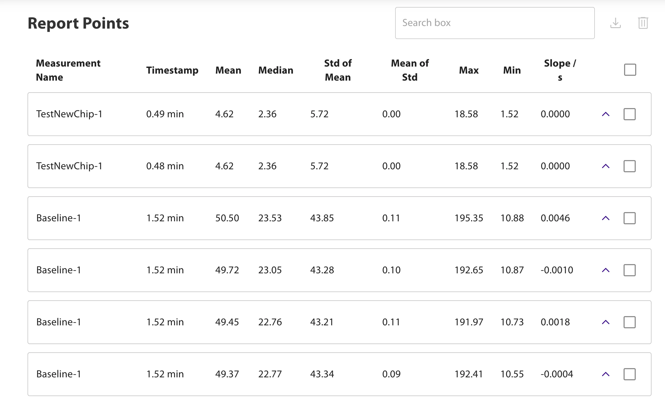
The table shows the measurement, description, injection group, timestamp, and median for each point. Show Details adds the mean, median, standard deviations, minimum, maximum, slope, delta, and metadata in compact sections, with heatmaps for the per-sensor statistics. The page exports a ZIP holding an overall and a per-sensor CSV.

Every spread reported here — the standard deviations and the boxplots — is taken across the molograms of one measurement at that time point. None of them is a fit uncertainty, and none is a standard error over independent samples. Two report points can therefore differ by more than their intervals suggest is likely, and still come from one preparation measured twice.

To compare them, enable batch operations, select saved report points of the same quantity, and choose Plot Selected. Their per-sensor median distributions are drawn as vertical boxplots, one box per selected report point.

These distributions describe the plotted data and nothing wider: sensors from one chip are technical observations, not independent biological replicates. Claims about a sample population still need independent measurements, chips, or donors, as the study design requires.

Interpreting a comparison

Compare the separation between negative and expected-response groups, not only the group averages — the individual sensor values are what reveal spread and outliers. When using the statistical brackets, select the intended reference first; every later selection is compared against it.
Check whether the ranking survives a change of chip or reagent batch. A reproducible rank on a shifted response scale is a different result from a changed biological conclusion.
Treat a responding negative sample, or a dilution series that is not monotonic, as a reason to investigate specificity, sample assignment and assay design — not as something to force back into the expected order.
Analyze direct and amplified readouts separately. A secondary reagent may improve separation, but it adds a binding step and its own variability.

Report point table listing each configured point with its time, value and sensor spread

Configure Report Points

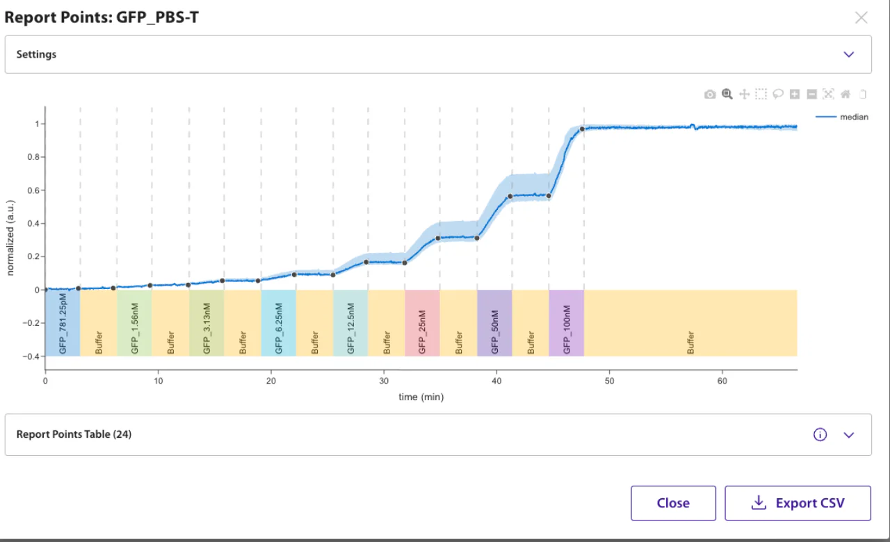
Report Points dialog showing the median trace with a shaded spread band, report point markers at the end of each injection, and the collapsed report points table — The dialog plots the median across sensors with a band for their spread, and marks each configured report point on the trace. The collapsed table below lists every point the current settings produce.

The Configure Report Points dialog previews the report points for a measurement before you rely on them. Open it from a plot on the Perform page, or from the More actions menu of any entry in a project's Processed Data table. When opened from processed data, the entry's cleanup actions are applied first, so the plot (with report-point markers), the Report Points Table, and the export all reflect the processed (cleaned) data. In that mode the phase comes from the processed-data selection and the plot shows the consensus (median) trace; holograms, injection-type settings, and the Near-zero threshold remain editable.

For raw measurements, the Phase filter accepts several phases at once; an empty selection includes every phase. The compact Report Points Table shows the report-point type, injection, start time, value, and delta. Open Show Details to inspect the time window, slope, cleanup cycle, sensor heatmap, and sensor-value boxplot.

To compare several samples or ligands after correcting for surface loading, add a Normalize → Normalize to immobilization levels cleanup action to the processed data first, then open this dialog from that entry. The normalization is carried into the plot, the automatic report points, the details and the export, so every value compared later comes from the same processed data.

CSV export

The dialog-level Export CSV button exports all sensor values alongside the consensus summary: the file contains one row per report point and sensor, each with its own mean, median, standard deviation, maximum, minimum, and slope, plus the report point's consensus (over-all-sensors) median, mean, and slope repeated on every row. Every row also carries the measurement name, sensor name, ligand name, the report-point timestamp, and the selectedtime window (s). The per-sensor mean is the arithmetic mean of that sensor's values inside this window; the consensus mean is then the mean of the per-sensor means. This makes it possible to trace every exported mean back to the interval used for its calculation while the consensus median remains available.

The Report Points Table's View column keeps a Show Details action for each row. It opens a per-report-point view with a sensor heatmap, a sensor-value boxplot, and a CSV export containing only that report point's per-sensor rows. To compare distributions, select one or more checkboxes in the same column and click Compare boxplots; every selected report point appears as a separate box in one chart. The comparison dialog shows the measurement name and one box per selected report point. The horizontal axis uses injection names, falling back to the injection group or "Manual" when no name is available. Hover over a box in the preview or interactive HTML export to see the report-point type, time, cycle when available, median, and sensor count.

The comparison dialog can export an interactive HTML plot, a high-resolution PNG image with the same concise axis labels, or the selected points' complete per-sensor CSV data.

Save to project

Automatically detected report points can be saved so they persist and appear on the Report Points page. Select one or more in the View column; Compare boxplots and Save to project appear together.

Where they go. Opened inside a project, they save to it directly; otherwise you pick the target project from a dropdown. Saving also adds the source measurement to that project's Raw Data, so a report point always has its underlying measurement available.
Duplicates. If the selection contains report points already in the project, a message states how many. Saving skips those, reports how many were skipped, and creates every new one. Saving a report point to another project does not prevent saving it to this one.
Partial failure. Only the report points that failed stay selected, ready to retry.

Report Point Calculations

Where the numbers come from. The consensus trace is the median across sensors at each time point, drawn here over the spread of the individual sensors. Value is read from the consensus trace at the report-point timestamp, delta is the difference from the previous report point in the sequence, and slope is fitted inside the window on every sensor separately and then averaged — so a wide band moves the slope even when the median looks clean.

For each report point the software evaluates the selected time window (for example the configured 5-second window near an injection end). Two computations produce its numbers, and they can differ slightly.

The preview table and the markers on the plot are read from the consensus trace — the median across the selected sensors at each time point:

Value: the consensus trace at the report-point timestamp.
Slope: the mean of the per-sensor slopes (a linear regression per sensor, averaged across sensors).
Delta: the difference from the previous row's value. On Capture Level and Binding rows the dialog also checks the consensus trace between the two points for a dip that approaches zero and recovers; if it finds one, the row is tagged Possible zero crossing and the delta is taken as sign-inverted. The Near-zero threshold (default 5 pg/mm², up to 15 pg/mm²) sets how close to zero that dip must come, and changes only the preview delta and the tag.

Saved report points, Show Details, the boxplots and every CSV are computed per sensor over the window and then aggregated across sensors:

Median (the saved value): the median across sensors of each sensor's window median.
Mean: the mean across sensors of each sensor's window mean.
Std of mean: the spread between sensors of those per-sensor means. Mean of std is instead the average within-window noise of the sensors.
Slope: the median across sensors of the per-sensor slopes.
Delta: the consensus trace at the end of the window minus the lowest consensus value in the 20 seconds before the injection starts; empty when the point lies outside an injection.

A preview row's value and slope can therefore differ slightly from the saved point's median and slope, and its delta is a different quantity.

Automatic Report Points

When viewing a measurement with injections, report points can be generated automatically based on injection type:

Type	Placed on	What it captures
Capture Level	Immobilization injections	Amount of ligand captured on the surface.
Binding Start	Association injections	Placed at the minimum value in the 20-second window before the injection starts — the baseline reference.
Binding	Association injections	Placed near the injection end.
Stability Point	Dissociation injections	Placed at the first timestamp where the signal drops by 5% relative to the previous Binding Start (or the baseline if no Binding Start exists) — marks the onset of dissociation.